mvndist.py, which recomputes what the entry states: the script block by block · open in ColabDictionary of Applied Machine Learning: 147 machine-learning terms, each with a definition, a figure, citations and a Python demo · All terms · Demos · Start here
Updated on 2026-11-20
Readiness 88/100
See also Gaussian random variable mean covariance matrix eigenvalue eigenvector maximum likelihood independent and identically distributed assumption empirical risk minimization Gaussian mixture model linear regression squared error loss linear discriminant analysis
The multivariate normal distribution is the probability distribution of a Gaussian random vector in $\mathbb{R}^{d}$, determined by a mean vector and a covariance matrix. Its probability density function (pdf) is proportional to the exponential of a negative quadratic form in the inverse of the covariance matrix, so its level sets are ellipsoids centered at the mean vector with axes along the eigenvectors of the covariance matrix and half-axes proportional to the square roots of its eigenvalues. The family is closed under affine maps and under conditioning, and among all random vectors with a given covariance matrix the Gaussian one has the largest differential entropy. The maximum likelihood estimates of the two parameters from a dataset are the sample mean and the sample covariance matrix, in closed form. When the covariance matrix is singular, no pdf exists and the random vector is confined to an affine subspace. In machine learning (ML), the multivariate normal distribution is the component of a Gaussian mixture model (GMM), the probabilistic model for the noise behind the squared error loss, and the class-conditional probability distribution behind linear discriminant analysis (LDA).
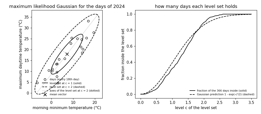
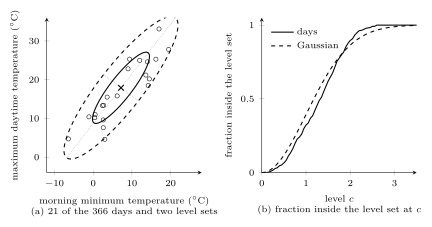
mvndist.py, which recomputes what the entry states: the script block by block · open in ColabB-dataConsider the $366$ days of $2024$ at Krems an der Donau, each a data point with a feature vector ${\mathbf x} \in \mathbb{R}^{2}$ that holds the morning minimum and the maximum daytime temperature of the day. A warm morning usually comes with a warm afternoon, so the days form an elongated cloud around their mean vector (Fig. 1(a)). The multivariate normal distribution is a probabilistic model for such feature vectors that describes this picture with two parameters (Anderson, 2003, Sect. 2.3; Bishop, 2006, Sect. 2.3). A mean vector ${\boldsymbol \mu} \in \mathbb{R}^{d}$ locates the center of the cloud, and a covariance matrix ${\mathbf C} \in \mathbb{R}^{d \times d}$ fixes its spread along every direction. The multivariate normal distribution is denoted by $\mathcal{N}\left({\boldsymbol \mu},{\mathbf C}\right)$, and a random vector with this probability distribution is a Gaussian random vector.
For an invertible covariance matrix ${\mathbf C}$, which is then positive definite (pd), the multivariate normal distribution has the probability density function (pdf) (Bishop, 2006, Sect. 2.3, Eq. (2.43)) \begin{equation} \label{equ_mvndist_pdf_dict} \mathcal{N}\left({\mathbf x} \,;\, {\boldsymbol \mu}, {\mathbf C}\right) = \frac{1}{(2\pi)^{d/2} \sqrt{\det({\mathbf C})}} \exp\Big( -\frac{1}{2} ({\mathbf x} - {\boldsymbol \mu})^{\top} {\mathbf C}^{-1} ({\mathbf x} - {\boldsymbol \mu}) \Big) \quad \text{for } {\mathbf x} \in \mathbb{R}^{d} \text{.} \end{equation} The exponent is a quadratic form in the inverse ${\mathbf C}^{-1}$, the precision matrix. The pdf \(\eqref{equ_mvndist_pdf_dict}\) is largest at ${\boldsymbol \mu}$ and falls off with the value of this quadratic form; the factor in front of the exponential, which contains the determinant of ${\mathbf C}$, makes it integrate to one. A random vector with the pdf \(\eqref{equ_mvndist_pdf_dict}\) has mean vector ${\boldsymbol \mu}$ and covariance matrix ${\mathbf C}$, which is what the two symbols are named for (Bishop, 2006, Sect. 2.3, Eqs. (2.59)–(2.64)). For $d = 1$, the pdf \(\eqref{equ_mvndist_pdf_dict}\) is the pdf of a Gaussian random variable (Gaussian RV) with mean $\mu$ and variance $\sigma^{2}$.
B-ellipseA level set of the pdf \(\eqref{equ_mvndist_pdf_dict}\) is the set of feature vectors at which the quadratic form takes a given value $c^{2}$, for some positive number $c$, \begin{equation} \label{equ_mvndist_levelset_dict} \big\{ {\mathbf x} \in \mathbb{R}^{d} : ({\mathbf x} - {\boldsymbol \mu})^{\top} {\mathbf C}^{-1} ({\mathbf x} - {\boldsymbol \mu}) = c^{2} \big\} \text{.} \end{equation} The covariance matrix is a symmetric matrix and admits a spectral decomposition ${\mathbf C} = \mathbf{V} \boldsymbol{\Lambda} \mathbf{V}^{\top}$, with orthonormal eigenvectors as the columns of $\mathbf{V}$ and the eigenvalues $\lambda_{1} \geq \ldots \geq \lambda_{d} > 0$ on the diagonal of $\boldsymbol{\Lambda}$. The level set \(\eqref{equ_mvndist_levelset_dict}\) is then an ellipsoid centered at ${\boldsymbol \mu}$, whose axes point along the eigenvectors and whose half-axis along the $j$th eigenvector has length $c \sqrt{\lambda_{j}}$ (Bishop, 2006, Sect. 2.3, Eqs. (2.44)–(2.52), Fig. 2.7). On it, the pdf equals $\exp(-c^{2}/2)$ times its value at ${\boldsymbol \mu}$. Fig. 1(a) shows the level sets at $c = 1$ and $c = 2$ for the days at Krems. The eigenvalues are $130.9$ and $7.9$ squared degrees Celsius, so the level set at $c = 2$ has half-axes of $22.9$ and $5.6$ degrees Celsius. Its major axis points along the eigenvector $(0.61, 0.79)^{\top}$, the direction in which minimum and maximum rise together.
B-coverageThe probability that a Gaussian random vector lies inside the level set \(\eqref{equ_mvndist_levelset_dict}\) depends on $c$ and $d$ only: the quadratic form of a Gaussian random vector has a chi-squared distribution with $d$ degrees of freedom (Anderson, 2003, Thm. 3.3.3). For $d = 2$, this probability is $1 - \exp(-c^{2}/2)$, that is, $39.3$ percent at $c = 1$, $86.5$ percent at $c = 2$, and $98.9$ percent at $c = 3$. Fig. 1(b) compares these values with the fraction of the days at Krems inside each level set: $32.2$, $89.6$, and $100$ percent. The days are spread along the major axis more evenly than a Gaussian random vector would be, since the seasons move a day along this axis. Only $59.8$ percent of them lie within one standard deviation of the mean along it, against $68.3$ percent for a Gaussian random vector, and no day lies beyond $c = 2.6$. A Gaussian mixture model (GMM) with two components, one for the cold and one for the warm days, describes such a cloud better than a single multivariate normal distribution.
Every Gaussian random vector is an affine function of a standard normal random vector ${\mathbf z} \in \mathbb{R}^{\ell}$, whose entries are independent and identically distributed (i.i.d.) standard Gaussian RVs: ${\mathbf x} = {\mathbf A} {\mathbf z} + {\boldsymbol \mu}$ with a matrix ${\mathbf A} \in \mathbb{R}^{d \times \ell}$, and then ${\mathbf C} = {\mathbf A} {\mathbf A}^{\top}$ (Anderson, 2003, Sect. 2.4). This construction also covers a singular covariance matrix, for which the pdf \(\eqref{equ_mvndist_pdf_dict}\) is undefined. The random vector is then confined to an affine subspace, the column space of ${\mathbf A}$ shifted by ${\boldsymbol \mu}$, which has volume zero in $\mathbb{R}^{d}$, so no pdf on $\mathbb{R}^{d}$ exists (Anderson, 2003, Sect. 2.4; Lapidoth, 2017, Ch. 23). A singular covariance matrix arises whenever one feature is an affine function of the others. Appending the daily temperature range, the maximum minus the minimum, as a third feature of a day at Krems yields a covariance matrix of rank two, and the three-dimensional feature vectors lie on a plane.
B-linearTwo properties make the multivariate normal distribution the default probabilistic model for numeric feature vectors. First, the family is closed under affine maps (Anderson, 2003, Thm. 2.4.5): for every matrix ${\mathbf B} \in \mathbb{R}^{q \times d}$ and every vector ${\mathbf c} \in \mathbb{R}^{q}$, \begin{equation} \label{equ_mvndist_affine_dict} {\mathbf x} \sim \mathcal{N}\left({\boldsymbol \mu},{\mathbf C}\right) \quad \text{implies} \quad {\mathbf B} {\mathbf x} + {\mathbf c} \sim \mathcal{N}\left({\mathbf B} {\boldsymbol \mu} + {\mathbf c},{\mathbf B} {\mathbf C} {\mathbf B}^{\top}\right) \text{.} \end{equation} Choosing ${\mathbf B}$ to select some entries of ${\mathbf x}$ shows that every marginal distribution of a multivariate normal distribution is again a multivariate normal distribution (Bishop, 2006, Sect. 2.3.2). For the days at Krems, the daily temperature range is the affine map \(\eqref{equ_mvndist_affine_dict}\) with ${\mathbf B} = (-1, 1)$ and ${\mathbf c} = 0$; under the probabilistic model, it has mean $10.7$ and variance ${\mathbf B} {\mathbf C} {\mathbf B}^{\top} = 19.7$ squared degrees Celsius. The family is also closed under conditioning. Given the values of some entries of ${\mathbf x}$, the conditional probability distribution of the remaining entries is a multivariate normal distribution. Its mean is an affine function of the given values, and its covariance matrix does not depend on them (Anderson, 2003, Thm. 2.5.1; Bishop, 2006, Sect. 2.3.1). Consider $d = 2$, and write $C_{1,1}$, $C_{1,2}$, and $C_{2,2}$ for the entries of the covariance matrix and $\mu_{1}$ and $\mu_{2}$ for the entries of the mean vector. The conditional probability distribution of $x_{2}$, given $x_{1}$, is then \begin{equation} \label{equ_mvndist_cond_dict} \mathcal{N}\left(\mu_{2} + \frac{C_{1,2}}{C_{1,1}} (x_{1} - \mu_{1}),C_{2,2} - \frac{C_{1,2}^{2}}{C_{1,1}}\right) \text{.} \end{equation} The conditional mean in the conditional probability distribution \(\eqref{equ_mvndist_cond_dict}\) is the prediction of the maximum temperature from the minimum with the smallest risk under the squared error loss, and it is linear in $x_{1}$ (see linear regression). For the days at Krems, it is the line learned by least squares, with slope $1.10$, and the conditional standard deviation is $4.4$ degrees Celsius. Second, among all random vectors with the covariance matrix ${\mathbf C}$, the Gaussian random vector has the largest differential entropy (Cover and Thomas, 2006, Thm. 8.6.5). When only the mean vector and the covariance matrix are known, the multivariate normal distribution is therefore the least restrictive probabilistic model.
The parameters ${\boldsymbol \mu}$ and ${\mathbf C}$ are learned from a dataset $\mathcal{D} = \{{\mathbf x}^{(1)}, \ldots, {\mathbf x}^{(m)}\}$ by maximum likelihood. Under the independent and identically distributed assumption (i.i.d. assumption), the data points are realizations of i.i.d. random vectors ${\mathbf x}^{(r)} \sim \mathcal{N}\left({\boldsymbol \mu},{\mathbf C}\right)$. The loss incurred by a data point is the negative logarithm of the pdf \(\eqref{equ_mvndist_pdf_dict}\) at its feature vector, and the average of this loss over $\mathcal{D}$ is the empirical risk of the pair $({\boldsymbol \mu}, {\mathbf C})$. Minimizing it is empirical risk minimization (ERM) over the hypothesis space of all pdfs \(\eqref{equ_mvndist_pdf_dict}\). The minimizer is available in closed form, so no iterative algorithm is needed (Anderson, 2003, Thm. 3.2.1; Bishop, 2006, Sect. 2.3.4, Eqs. (2.121)–(2.122)): \begin{equation} \label{equ_mvndist_mle_dict} \widehat{\boldsymbol \mu} = \frac{1}{m} \sum_{r=1}^{m} {\mathbf x}^{(r)} \quad \text{and} \quad \widehat{{\mathbf C}} = \frac{1}{m} \sum_{r=1}^{m} \big( {\mathbf x}^{(r)} - \widehat{\boldsymbol \mu} \big) \big( {\mathbf x}^{(r)} - \widehat{\boldsymbol \mu} \big)^{\top} \text{.} \end{equation} The estimates \(\eqref{equ_mvndist_mle_dict}\) are the sample mean and the sample covariance matrix of $\mathcal{D}$ with the divisor $m$; under the i.i.d. assumption, the sample covariance matrix is smaller than ${\mathbf C}$ on average by the factor $(m - 1)/m$ (Bishop, 2006, Sect. 2.3.4, Eq. (2.124)). For the days at Krems, the estimates \(\eqref{equ_mvndist_mle_dict}\) are $\widehat{\boldsymbol \mu} = (7.2, 17.9)^{\top}$ and a sample covariance matrix with variances $54.2$ and $84.6$ and covariance $59.6$, all in squared degrees Celsius; the correlation coefficient of minimum and maximum temperature is $0.88$. The sample covariance matrix has rank at most $m - 1$, so with fewer than $d + 1$ data points it is singular and the pdf \(\eqref{equ_mvndist_pdf_dict}\) with these estimates is undefined. A common remedy replaces $\widehat{{\mathbf C}}$ by a weighted average of it and a positive multiple of the identity matrix (Hastie et al., 2009, Sect. 4.3.1, Eq. (4.14)). This shrinks the hypothesis space to covariance matrices whose eigenvalues are bounded away from zero, one of the routes that regularization distinguishes.
B-plotThe multivariate normal distribution is used throughout machine learning (ML).
A GMM draws the feature vector of a data point from
one of $k$ multivariate normal distributions, so each
cluster of a soft clustering is a mean
vector with a covariance matrix, drawn as an ellipse
(Bishop, 2006, Sect. 9.2). In regression, the
label of a data point is modeled as the value of a
hypothesis plus a Gaussian random variable (RV) with mean zero.
Maximum likelihood estimation of the hypothesis is then
ERM with the squared error loss, so linear regression by
least squares assumes this probabilistic model for the
label (Bishop, 2006, Sects. 1.2.5 and 3.1.1). In
classification, modeling the feature vector of each class
by a multivariate normal distribution and comparing the
logarithms of the pdfs \(\eqref{equ_mvndist_pdf_dict}\) yields
a classifier with the smallest risk under that
probabilistic model. With one covariance matrix shared by all classes, the
quadratic terms cancel and the decision boundary is a
hyperplane, which is linear discriminant analysis (LDA). With a covariance matrix per class,
the decision boundary is a quadratic surface
(Bishop, 2006, Sect. 4.2.1; Hastie et al., 2009, Sect. 4.3,
Eqs. (4.9) and (4.12)).
pythondemos/mvndist.py
Synonyms: multivariate Gaussian distribution, joint normal distribution, jointly Gaussian distribution.
See also: Gaussian random variable, normal distribution, random vector, mean, covariance matrix, probability density function, precision matrix, spectral decomposition, eigenvalue, eigenvector, standard normal random vector, maximum likelihood, sample mean, sample covariance matrix, independent and identically distributed assumption, empirical risk minimization, Gaussian mixture model, linear regression, squared error loss, linear discriminant analysis, differential entropy, probabilistic model.
@misc{dictml_mvndist,
  author = {Jung, Alexander},
  editor = {Olioumtsevits, Konstantina and Schnoor, Ekkehard},
  title = {multivariate normal distribution},
  howpublished = {Dictionary of Applied Machine Learning (course edition)},
  year = {2026},
  doi = {10.5281/zenodo.21569296},
  note = {ISBN 978-952-64-3013-3, CC BY 4.0, retrieved 2026-11-20},
  url = {https://dictionaryofml.org/terms/mvndist.html}
}