lda.py, which recomputes what the entry states: the script block by block · open in ColabDictionary of Applied Machine Learning: 147 machine-learning terms, each with a definition, a figure, citations and a Python demo · All terms · Demos · Start here
Updated on 2026-11-20
Readiness 88/100
See also principal component analysis feature learning feature transformation dimensionality reduction binary classification linear classifier decision boundary kernel method logistic regression
Linear discriminant analysis (LDA) learns a linear feature transformation that replaces the feature vector of a data point by one feature, chosen so that the two label values of a binary classification problem are told apart as well as possible. The criterion is the Fisher criterion, the ratio of the between-class to the within-class scatter of the new feature. The direction attaining its maximum is obtained by solving one linear system, so LDA is a closed form rather than an iterative method. The two scatter matrices add up to the sample covariance matrix, the matrix whose quadratic form principal component analysis (PCA) maximizes, so PCA keeps the direction of largest total sample variance while LDA weighs the two parts against each other. A direction can carry nearly all of the sample variance and nearly none of the between-class part. With more than two label values, LDA delivers at most one direction fewer than there are values. The name also denotes the classifier that reaches the same direction from a multivariate normal distribution per label value with one shared covariance matrix.
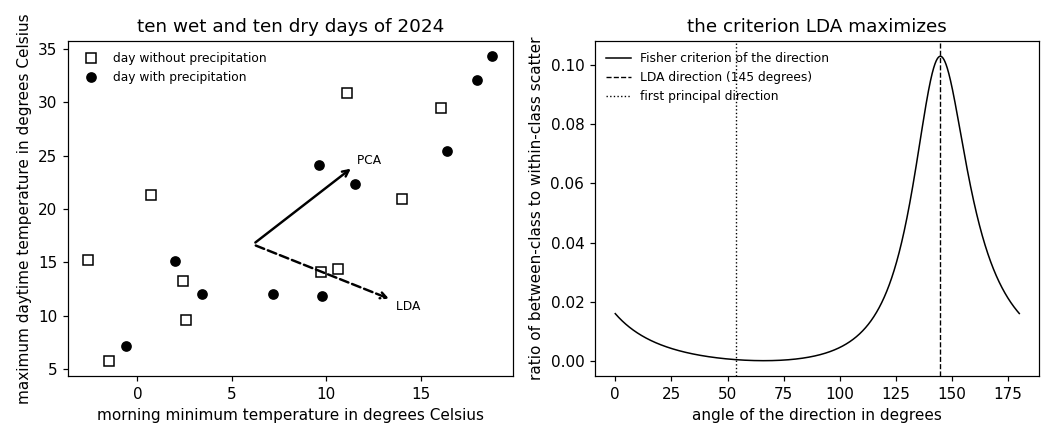
lda.py, which recomputes what the entry states: the script block by block · open in ColabB-dataA weather station at Krems an der Donau (Austria) records the morning minimum and the maximum daytime temperature of each day, and a forecaster wants one number per day that tells the days with precipitation from the dry ones. The two temperatures move together: a cold day is cold in the morning and in the afternoon, a warm day is warm in both. That shared swing is the direction along which the days vary most, and it is the direction principal component analysis (PCA) keeps. It is also close to useless for the question asked, because it says how warm a day was and not whether it rained. LDA produces one number per day as well, and it chooses the direction from the labels.
B-scatterLDA is a feature learning method for binary classification. Consider a training set $\mathcal{D}^{(\rm train)} = \big\{ ({\mathbf x}^{(1)}, y^{(1)}), \ldots, ({\mathbf x}^{(m)}, y^{(m)}) \big\}$ of sample size $m$, with feature vectors ${\mathbf x}^{(r)} \in \mathbb{R}^{d}$ and labels $y^{(r)} \in \{-1,+1\}$. LDA learns a linear feature transformation \[\phi^{({\mathbf w})}: \mathbb{R}^{d} \rightarrow \mathbb{R}: {\mathbf x} \mapsto {\mathbf w}^{\top} {\mathbf x} \text{,}\] which replaces the $d$ raw features of a data point by the single new feature $\phi^{({\mathbf w})}({\mathbf x})$. The labels enter through two matrices. Let $\widehat{{\boldsymbol \mu}}^{(c)}$ be the sample mean of the feature vectors carrying the label value $c$, and $p_{c}$ the fraction of the training set that carries it. The sample mean of all feature vectors is then $\widehat{\boldsymbol \mu} = \sum_{c \in \{-1,+1\}} p_{c} \widehat{{\boldsymbol \mu}}^{(c)}$. The two matrices are (Hastie et al., 2009, Sect. 4.3.3): \begin{equation} \label{equ_lda_scatter_dict} \mathbf{S} := \frac{1}{m} \sum_{c \in \{-1,+1\}} \sum_{r \, : \, y^{(r)} = c} \big( {\mathbf x}^{(r)} - \widehat{{\boldsymbol \mu}}^{(c)} \big) \big( {\mathbf x}^{(r)} - \widehat{{\boldsymbol \mu}}^{(c)} \big)^{\top} \text{,} \end{equation} \begin{equation} \label{equ_lda_between_dict} {\mathbf B} := \sum_{c \in \{-1,+1\}} p_{c} \big( \widehat{{\boldsymbol \mu}}^{(c)} - \widehat{\boldsymbol \mu} \big) \big( \widehat{{\boldsymbol \mu}}^{(c)} - \widehat{\boldsymbol \mu} \big)^{\top} \text{.} \end{equation} The within-class scatter matrix $\mathbf{S}$ averages the spread of the feature vectors around the sample mean of their own label value, and the between-class scatter matrix ${\mathbf B}$ measures how far the two sample means lie apart. Along a direction ${\mathbf w}$, the new feature has within-class sample variance ${\mathbf w}^{\top} \mathbf{S} {\mathbf w}$ and between-class sample variance ${\mathbf w}^{\top} {\mathbf B} {\mathbf w}$.
B-ldaThe criterion LDA maximizes is the ratio of the two, the Fisher criterion (Bishop, 2006, Sect. 4.1.4, Eq. (4.26); Fisher, 1936; Hastie et al., 2009, Sect. 4.3.3, Eq. (4.15)), \begin{equation} \label{equ_lda_fisher_dict} \max_{{\mathbf w} \in \mathbb{R}^{d} \, : \, \Vert {{\mathbf w}} \Vert = 1} \frac{{\mathbf w}^{\top} {\mathbf B} {\mathbf w}}{{\mathbf w}^{\top} \mathbf{S} {\mathbf w}} \text{.} \end{equation} A direction scores high when the two sample means are far apart on it and the days of one label value stay close together on it. The ratio of the two sample variances in the Fisher criterion \(\eqref{equ_lda_fisher_dict}\) does not change when ${\mathbf w}$ is rescaled, so the constraint costs nothing and what is learned is a direction. For an invertible $\mathbf{S}$, the maximizing direction is that of \begin{equation} \label{equ_lda_solution_dict} \widehat{{\mathbf w}} = \mathbf{S}^{-1} \big( \widehat{{\boldsymbol \mu}}^{(+1)} - \widehat{{\boldsymbol \mu}}^{(-1)} \big) \end{equation} (Bishop, 2006, Sect. 4.1.4, Eq. (4.30)). The LDA direction \(\eqref{equ_lda_solution_dict}\) is computed in closed form, by solving one linear system: LDA is not an iterative method, so no operator has its output as a fixed point.
The name also denotes a classifier, not only the feature transformation. Modeling each label value by a multivariate normal distribution with its own mean and one shared covariance matrix, and estimating these model parameters by maximum likelihood, gives a linear classifier whose decision boundary is a hyperplane with the normal vector \(\eqref{equ_lda_solution_dict}\) (Hastie et al., 2009, Sect. 4.3). The direction is the same, and the probabilistic model supplies the threshold that the Fisher criterion leaves open.
The difference from PCA is one matrix. The within-class scatter matrix \(\eqref{equ_lda_scatter_dict}\) and the between-class scatter matrix \(\eqref{equ_lda_between_dict}\) add up to the sample covariance matrix (Hastie et al., 2009, Sect. 4.3.3), \begin{equation} \label{equ_lda_decomp_dict} \mathbf{S} + {\mathbf B} = \widehat{{\mathbf C}} \text{.} \end{equation} The labels have disappeared from the sum \(\eqref{equ_lda_decomp_dict}\). PCA maximizes ${\mathbf w}^{\top} \widehat{{\mathbf C}} {\mathbf w}$ over the directions of unit norm, which is the total sample variance of the new feature and says nothing about which part of the sum \(\eqref{equ_lda_decomp_dict}\) it comes from. The Fisher criterion \(\eqref{equ_lda_fisher_dict}\) weighs the two parts against each other instead. A direction can therefore carry nearly all of the total sample variance and nearly none of the between-class part, which is what the opening example describes.
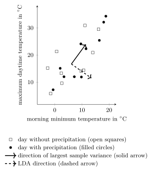
B-plotThat example is measurable. The training set holds the $1461$
days of $2020$ to $2023$ at Krems, each with the morning minimum
and the maximum daytime temperature as its two features
and the label $+1$ when precipitation was recorded. The
eigenvector of $\widehat{{\mathbf C}}$ belonging to its
largest eigenvalue carries $93$ percent of the total
sample variance and reaches a Fisher
criterion of $0.00034$, while the LDA direction
\(\eqref{equ_lda_solution_dict}\) reaches $0.103$, larger by a factor
of $303$. The two directions are $89$ degrees apart, so what the
labels depend on lies almost exactly along the direction
PCA ranks last (Fig. 1). The
LDA direction weighs
the two features with opposite signs, $(0.817, -0.577)$,
so its new feature is large on a day whose temperature
changed little between morning and afternoon, which is what cloud
cover does.
pythondemos/lda.py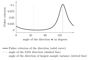
pythondemos/lda.py
Where a linear combination is not enough, the answer is to run LDA on an enlarged feature vector that also holds the squares and the products of the raw features. A hyperplane in the feature space of the enlarged feature vector is a curved decision boundary in the feature space of the raw features (Hastie et al., 2009, Sect. 12.5), and a kernel method is the general form of the step. What LDA buys for the cost of solving one linear system is the factor of $303$ in the Fisher criterion \(\eqref{equ_lda_fisher_dict}\). Of the two single features at Krems, the one chosen from the labels gains $3.0$ percentage points on predicting the majority label value and the PCA feature gains $0.3$.
See also: principal component analysis, feature learning, feature transformation, dimensionality reduction, binary classification, linear classifier, sample covariance matrix, decision boundary, kernel method, logistic regression.
@misc{dictml_lda,
  author = {Jung, Alexander},
  editor = {Olioumtsevits, Konstantina and Schnoor, Ekkehard},
  title = {linear discriminant analysis (LDA)},
  howpublished = {Dictionary of Applied Machine Learning (course edition)},
  year = {2026},
  doi = {10.5281/zenodo.21569296},
  note = {ISBN 978-952-64-3013-3, CC BY 4.0, retrieved 2026-11-20},
  url = {https://dictionaryofml.org/terms/lda.html}
}