pythondemos/featlearn.py
Dictionary of Applied Machine Learning
Updated on 2026-09-19
Typeset PDF version — the authoritative form of this entry
Python demo — a script that recomputes what this entry states and prints one line per check
Feature learning is the task of learning, from a dataset, a feature transformation that turns the raw features of a data point into new features that make a subsequent learning task easier. A feature learning method is specified by the two feature spaces, by a hypothesis space of candidate feature transformations, and by a quantitative measure of how useful a feature transformation is, computed from a dataset that need not carry labels. Principal component analysis (PCA) learns a linear feature transformation to fewer features, judged by the linear reconstruction error, and an autoencoder obtains a nonlinear one by the same criterion. The hidden layers of a deep net form a chain of feature transformations learned jointly with the output layer, so that each layer builds its features from those of the previous one. Pretraining an encoder on unlabeled data points learns features that are reused across learning tasks. In weather forecasting, forty measurements from the five days before are turned into two learned features from which linear regression predicts the maximum temperature of the next day.
B-datasetConsider the task of forecasting the weather of tomorrow at a weather station from the measurements of the previous five days. Each day is a data point, its label is the maximum temperature of that day, and its raw features are the eight daily measurements (lowest, highest and mean air temperature, precipitation, sunshine duration, humidity, air pressure and wind speed) of each of the five previous days: a list of forty numbers. A point with forty coordinates cannot be drawn in a scatterplot. A feature transformation that delivers two new features from the forty raw ones places every day in a scatterplot, and a linear model of the two new features may already predict the label. Feature learning is the task of learning such a feature transformation from a dataset instead of designing it by hand.
Feature learning is the task of learning a feature transformation \[\featuretrafovec: \featurespace \rightarrow \featurespace', \qquad \featurevec \mapsto \vz \defeq \featuretrafovec(\featurevec) \text{.}\] The transformation reads in the raw feature vector $\featurevec \in \featurespace$ of a data point and delivers a new feature vector $\vz$ from a new feature space $\featurespace'$. A feature learning method is specified by three design choices: the two feature spaces $\featurespace$ and $\featurespace'$, a hypothesis space $\hypospace$ of candidate feature transformations, and a quantitative measure of how useful a specific $\featuretrafovec \in \hypospace$ is. The measure is computed from a dataset, which need not carry labels, and it need not be the dataset of the learning task at hand. A useful feature transformation is one that makes a subsequent learning task easier (Goodfellow et al., 2016, Ch. 15): the data points become separable by a linear model, fewer features suffice, or the features learned once serve several learning tasks. Alternative constructions of a feature transformation do not learn $\featuretrafovec$ (Goodfellow et al., 2016, Ch. 6). A kernel method fixes $\featuretrafovec$ through the choice of a kernel, with $\featurespace'$ the reproducing kernel Hilbert space (RKHS) $\hilbertspace_{\kernel}$ and $\vz = \kernelmap{\featurevec}{\cdot}$ never evaluated explicitly, and learns only a linear hypothesis on $\featurespace'$. A hand-designed $\featuretrafovec$ encodes domain knowledge instead of a dataset.
B-pcaPrincipal component analysis (PCA) is feature learning with $\featurespace \defeq \reals^{\featuredim}$, $\featurespace' \defeq \reals^{\featuredim'}$ for some $\featuredim' < \featuredim$, and the hypothesis space of linear maps, \[\hypospace \defeq \big\{ \featuretrafovec: \reals^{\featuredim} \rightarrow \reals^{\featuredim'}: \featurevec \mapsto \mW \featurevec \text{ with some } \mW \in \reals^{\featuredim' \times \featuredim} \big\} \text{.}\] The usefulness of a specific $\featuretrafovec(\featurevec) = \mW \featurevec$ is measured by the minimum linear reconstruction error on the dataset $\dataset = \big\{ \featurevec^{(1)}, \ldots, \featurevec^{(\samplesize)} \big\}$, \[\min_{\mR \in \reals^{\featuredim \times \featuredim'}} \sum_{\sampleidx=1}^{\samplesize} \normgeneric{\featurevec^{(\sampleidx)} - \mR \mW \featurevec^{(\sampleidx)}}{2}^{2} \text{,}\] and the rows of the best $\mW$ are the $\featuredim'$ eigenvectors of the sample covariance matrix with the largest eigenvalues (Hastie et al., 2009, Sect. 14.5.1). An autoencoder measures usefulness by the same reconstruction error but replaces the linear maps $\mW$ and $\mR$ by artificial neural networks (ANNs), so that the new features are obtained by a nonlinear feature transformation.
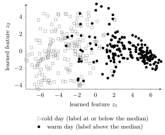
B-linregApplied to the weather example, PCA delivers the two learned
features of Fig. 1. The forty raw
features of the 361 days of 2024 at Krems, each scaled to zero sample mean and unit
sample variance because temperatures, precipitation and
pressure carry different units, are turned into two learned
features. Warm and cold days separate along the first
learned feature: 89 percent of the warm days have a positive
$z_{1}$ and 92 percent of the cold days a nonpositive one.
Linear regression on the two learned
features, after training on the days from January to
August, predicts the maximum temperature of the days from September
to December with a validation error of 13.5 (squared degrees Celsius),
against 10.2 for linear regression on all forty raw features and
110.9 for predicting the sample mean of the training
labels.
pythondemos/featlearn.py
See also: feature transformation, feature, feature space, hypothesis space, principal component analysis, autoencoder, dimensionality reduction, deep net, layer, pretraining.
@misc{dictml_featlearn,
  author = {Jung, Alexander and Olioumtsevits, Konstantina and Schnoor, Ekkehard},
  title = {feature learning},
  howpublished = {Dictionary of Applied Machine Learning (course edition)},
  year = {2026},
  doi = {10.5281/zenodo.21569296},
  note = {ISBN 978-952-64-3013-3, CC BY 4.0, retrieved 2026-09-19},
  url = {https://dictionaryofml.org/terms/featlearn.html}
}