hypothesis space

Typeset PDF version — the authoritative form of this entry

A hypothesis space $\hypospace$ is a set of hypothesis maps $\hypothesis: \featurespace \rightarrow \labelspace$ from a feature space into a label space. Every machine learning (ML) method uses an underlying hypothesis space, which is a subset of the set $\labelspace^{\featurespace}$ of all possible maps from $\featurespace$ into $\labelspace$. Available computational resources limit the size of $\hypospace$, which in turn shapes the method's computational cost and predictive behavior. The hypothesis space typically carries geometric structure: real-valued hypotheses can be compared via the deviation in their predictions on a reference dataset, and a parametric model inherits a geometric structure from the underlying parameter space $\paramspace$.

Definition

A weather service predicting tomorrow's maximum daytime temperature from today's morning temperature must commit to a set of candidate prediction maps: for example, all linear functions of the morning temperature. 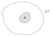This set of candidates is the hypothesis space of the method; more generally, every machine learning (ML) method commits to a specific hypothesis space $\hypospace$, the set from which it learns a single hypothesis $\learnthypothesis$. Formally, $\hypospace$ is a subset of the set $\labelspace^{\featurespace}$ of all possible maps from the feature space into the label space (see Fig. 1).

Figure 1 of the entry hypospace — Figure 1: Hypothesis space $\hypospace$ of an ML method as a restricted subset of the much larger set $\labelspace^{\featurespace}$ of all possible maps from the feature space $\featurespace$ into the label space $\labelspace$

Linear regression and other linear methods use the linear model as $\hypospace$, i.e., the set of all linear maps $\reals^{\featuredim} \rightarrow \reals$ (Shalev-Shwartz and Ben-David, 2014, Ch. 2). Another canonical example is %need to check citation again - maybe Sect. 2.3 for the first sentences? and linear regression is mentioned in Sect. 9.2 the set of input–output maps realizable by an artificial neural network (ANN) of fixed architecture, as the model parameters vary.

The choice of $\hypospace$ is a central design decision for an ML method. From an ML engineering perspective, it is guided by two factors. The first is the available computational resources, such as memory, processing time, and communication bandwidth. The second factor is the number of available data points, which limits the maximum size of $\hypospace$ that can be effectively trained without overfitting.

The size of the underlying $\hypospace$ is an important characteristic of an ML method. In principle, $\hypospace$ could be as large as $\labelspace^{\featurespace}$ itself. In practice, finite computational resources restrict an ML method to a much smaller subset $\hypospace$. The size of $\hypospace$ allows the anticipation of generalization before any training is carried out. A small $\hypospace$ typically incurs a small generalization gap, while a large $\hypospace$ is more prone to overfitting. For a finite $\hypospace$ we can use the cardinality as effective size. For an infinite $\hypospace$, an effective size can be quantified by the Vapnik–Chervonenkis dimension (VC dimension) or the Rademacher complexity.

The same $\hypospace$ can be used by different ML algorithms, such as empirical risk minimization (ERM) on a fixed training set, online learning on a stream of data points, or Bayesian inference that returns a posterior distribution over $\hypospace$ rather than a single hypothesis (Bishop, 2006, Sect. 1.2.3).

The word space (rather than set) reflects the fact that $\hypospace$ typically carries some geometric structure. In general, $\hypospace$ is not a vector space: the sum of two hypotheses in $\hypospace$ need not belong to $\hypospace$. What is more, there are hypothesis spaces that are not equipped with an algebraic structure at all, i.e., there is no meaningful way to add two hypotheses in $\hypospace$ or to multiply a hypothesis by a scalar.

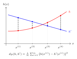
For real-valued hypotheses, two $\hypothesis, \hypothesis' \in \hypospace$ can be compared by their average squared prediction deviation on a reference dataset $\dataset = \{\featurevec^{(1)}, \ldots, \featurevec^{(\samplesize)}\}$, \[ \frac{1}{\samplesize} \sum_{\sampleidx=1}^{\samplesize} \big(\hypothesis(\featurevec^{(\sampleidx)}) - \hypothesis'(\featurevec^{(\sampleidx)})\big)^{2} \text{.} \] Fig. 2 illustrates this comparison: the two hypotheses are evaluated on the data points in $\dataset$ and the squared differences in their predictions are averaged. This construction is not meaningful for hypotheses with a finite label space, as used in classification methods. Instead, two such hypotheses can be compared by their disagreement rate on $\dataset$.

Figure 2 of the entry hypospace — Figure 2: Comparing two hypotheses $\hypothesis$ (red) and $\hypothesis'$ (blue) by their predictions at four scalar features $\feature^{(1)},\ldots,\feature^{(4)}$. The dashed segments mark the gap $\hypothesis(\feature^{(\sampleidx)}) - \hypothesis'(\feature^{(\sampleidx)})$ for each data point; the average of its square defines the distance $d_{\dataset}(\hypothesis,\hypothesis')$ between $\hypothesis$ and $\hypothesis'$

A parametric model $\hypospace = \{\hypothesis^{(\weights)} : \weights \in \paramspace\}$ inherits a geometric structure from the underlying parameter space $\paramspace \subseteq \mathbb{R}^{\dimlocalmodel}$. A norm on $\mathbb{R}^{\dimlocalmodel}$ induces the candidate distance $\metric{\hypothesis^{(\weights)}}{\hypothesis^{(\weights')}} \defeq \norm{\weights - \weights'}$ on $\hypospace$. When the parameterization $\weights \mapsto \hypothesis^{(\weights)}$ is injective, distinct weight vectors give distinct hypotheses, and this candidate distance is a genuine metric. The linear model $\hypospace = \{\hypothesis^{(\weights)}(\featurevec) = \weights^{\top} \featurevec : \weights \in \reals^{\featuredim}\}$ is a canonical example of an injective parameterization: distinct weight vectors $\weights$ produce distinct linear maps, so $\norm{\weights - \weights'}$ is a metric on $\hypospace$. When the parameterization is not injective, two distinct weight vectors $\weights \neq \weights'$ can represent the same hypothesis $\hypothesis^{(\weights)} = \hypothesis^{(\weights')}$. The distance $\norm{\weights - \weights'}$ is then strictly positive even though the two hypotheses coincide, so it is only a pseudo-metric. Permuting the hidden units of an ANN, for instance, changes $\weights$ but leaves $\hypothesis^{(\weights)}$ unchanged.

Synonyms: hypothesis class, model.

See also: hypothesis, model, map, linear model, parametric model, parameter space, metric, norm, empirical risk minimization, online learning, Bayesian inference, posterior distribution, Vapnik–Chervonenkis dimension, Rademacher complexity.

References

Shalev-Shwartz and Ben-David (2014). Understanding Machine Learning: From Theory to Algorithms. Cambridge Univ. Press.
Bishop (2006). Pattern Recognition and Machine Learning. Springer Science+Business Media.

Cite this entry

@misc{dictml_hypospace,
  author = {Jung, Alexander},
  title = {hypothesis space},
  howpublished = {Dictionary of Applied Machine Learning (course edition)},
  year = {2026},
  doi = {10.5281/zenodo.21569296},
  note = {ISBN 978-952-64-3013-3, CC BY 4.0, retrieved 2026-08-06},
  url = {https://dictionaryofml.org/terms/hypospace.html}
}