Dictionary of Applied Machine Learning
Updated on 2026-08-28
Typeset PDF version — the authoritative form of this entry
Online learning refers to machine learning (ML) methods that process data sequentially: at each discrete time instant a new data point arrives and the method updates its current model parameters, in contrast with solving empirical risk minimization (ERM) once over a fixed training set. The canonical update is a gradient step on the loss of the newest data point, which is online gradient descent (online GD). For data points that are realizations of independent and identically distributed (i.i.d.) random variables (RVs), the expected update is a gradient step on the risk, and online GD coincides with stochastic gradient descent (SGD) with batch size one. Performance is measured by the regret, the accumulated loss minus that of the best fixed model parameters in hindsight. With a suitably decaying learning rate, the average regret per round of online GD vanishes as the number of rounds grows.
A Finnish Meteorological Institute (FMI) weather station delivers one new data point every evening: the day's morning minimum and its maximum daytime temperature. A method that first collects a complete training set never starts forecasting. Online learning instead updates the hypothesis every day, using the newest data point (Jung, 2022, Sect. 4.7).
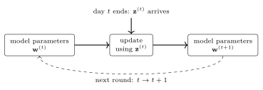
Online learning refers to machine learning (ML) methods that process data
sequentially: data points $\datapoint^{(\timeidx)}$ arrive at
discrete time instants $\timeidx = 1, 2, \ldots$, and at each
instant the method updates its current model parameters
$\weights^{(\timeidx)}$, or hypothesis
$\hypothesis^{(\timeidx)}$, using $\datapoint^{(\timeidx)}$
(Fig. 1). This contrasts with solving
empirical risk minimization (ERM) once over a fixed training set. The time index is also
the iteration index: one new data point means one update.
The quality of an online method is measured in hindsight. After $\nriter$ rounds, the accumulated loss $\sum_{\timeidx=1}^{\nriter} \lossfunc{\datapoint^{(\timeidx)}}{\weights^{(\timeidx)}}$ is compared with the accumulated loss of the best fixed model parameters chosen after all data points have been seen; the difference is the regret. With a suitably decaying learning rate, online GD keeps the average regret per round vanishing as $\nriter$ grows (Hazan, 2022).
For linear regression on the temperature stream, the model parameters that minimize the average squared error loss over all days up to time $\timeidx$ need not be recomputed from scratch each day: the solution at time $\timeidx + 1$ reuses the matrix computations of time $\timeidx$ (Jung, 2022, Sect. 4.7).
See also: online gradient descent, online algorithm, stochastic gradient descent, gradient descent, gradient step, empirical risk minimization, regret, risk, linear regression.
@misc{dictml_onlinelearning,
  author = {Jung, Alexander and Olioumtsevits, Konstantina and Schnoor, Ekkehard},
  title = {online learning},
  howpublished = {Dictionary of Applied Machine Learning (course edition)},
  year = {2026},
  doi = {10.5281/zenodo.21569296},
  note = {ISBN 978-952-64-3013-3, CC BY 4.0, retrieved 2026-09-19},
  url = {https://dictionaryofml.org/terms/onlinelearning.html}
}