Dictionary of Applied Machine Learning

gradient descent

Typeset PDF version — the authoritative form of this entry

Definition

Many machine learning (ML) applications amount to solving an optimization problem: an objective function $f: \reals^{\nrfeatures} \rightarrow \reals$ measures the quality of the vector $\weights \in \reals^{\nrfeatures}$ of model parameters, which is the optimization variable. When training a deep net for image recognition, for example, $f(\weights)$ is the average loss incurred by the network on a training set of labeled images.

In many important cases, the objective function is differentiable: at every point $\weights$ there exists a gradient $\nabla f(\weights) \in \reals^{\nrfeatures}$, the vector of partial derivatives of $f$ at $\weights$, which determines a local linear approximation of $f$ (see differentiable).

GD uses this local linear approximation to iteratively improve the current choice of the model parameters: starting from an initialization $\weights^{(0)}$, GD generates a sequence of estimates $\weights^{(0)}, \weights^{(1)}, \weights^{(2)}, \ldots$ that ideally converge to a minimum of $f$. GD and its variants are the standard solvers for model training in deep learning (Goodfellow et al., 2016).

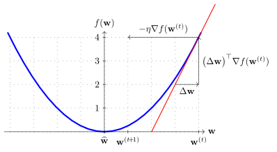
At each iteration $\iteridx$, GD refines the current estimate $\weights^{(\iteridx)}$ by stepping in the direction of steepest descent of the local linear approximation to $f$ at $\weights^{(\iteridx)}$. This direction is the negative gradient $\nabla f(\weights^{(\iteridx)})$, giving the update \begin{equation} \label{equ_def_GD_step_dict} \weights^{(\iteridx+1)} = \weights^{(\iteridx)} - \lrate \nabla f(\weights^{(\iteridx)}) \text{,} \end{equation} where $\lrate > 0$ is a step size. For a sufficiently small $\lrate$, each step decreases the function value, $f(\weights^{(\iteridx+1)}) \le f(\weights^{(\iteridx)})$, with strict decrease whenever $\nabla f(\weights^{(\iteridx)}) \neq \mathbf{0}$ (Boyd and Vandenberghe, 2004, Sect. 9.3). Fig. 1 illustrates a single GD step.

Consider shrinking the step size $\lrate$ in the GD step \(\eqref{equ_def_GD_step_dict}\) toward zero. This results in iterates $\weights^{(\iteridx)}$ becoming approximately the values of a continuous-time trajectory $\weights(\tau)$. This trajectory satisfies the ordinary differential equation $\dot{\weights}(\tau) = -\nabla f(\weights(\tau))$, which is known as gradient flow. In particular, GD is the explicit Euler discretization of this gradient flow with step $\lrate$ (Helmke and Moore, 1994). Indeed, replacing the time derivative $\dot{\weights}(\tau)$ by the difference quotient $\big(\weights^{(\iteridx+1)} - \weights^{(\iteridx)}\big)/\lrate$ recovers the update \(\eqref{equ_def_GD_step_dict}\). 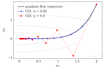Fig. 2 illustrates how, for a small step size, the GD iterates closely follow the gradient flow trajectory.

Assume, moreover, that $f$ is $\mu$-strongly convex, i.e., the function $f(\weights) - (\mu/2) \norm{\weights}^{2}$ is still convex, so the curvature of $f$ is at least $\mu > 0$ in every direction. Then $\gdstep{\lrate}$ is a contractive operator with respect to the same norm, \[ \norm{\gdstep{\lrate}(\weights) - \gdstep{\lrate}(\weights')} \le (1 - \mu\lrate)\,\norm{\weights - \weights'} \text{.} \] In this case, Banach's fixed-point theorem gives a unique fixed point $\widehat{\weights}$ (the minimizer of $f$) to which GD converges at a geometric rate (Boyd and Vandenberghe, 2004; Nesterov, 2004). For linear regression, these properties are explicit: the gradient of the average squared error loss is an affine function of $\weights$, and the contraction factor of $\gdstep{\lrate}$ is governed by the eigenvalues of the matrix $\featuremtx^{\top}\featuremtx$. Here, $\featuremtx$ denotes the feature matrix, whose rows are the feature vectors of the data points in the training set (see linear regression).

How fast GD converges depends on the curvature of $f$, as quantified by the constants $L$ and $\mu$ above. Let $\widehat{\weights}$ be a minimizer and $f^{\star} = f(\widehat{\weights})$. For convex $f$ with $L$-Lipschitz gradient and the constant step size $\lrate = 1/L$ (Beck, 2017, Ch. 10; Bubeck, 2015, Th. 3.3), \[ f\big(\weights^{(\nriter)}\big) - f^{\star} \le \frac{L\,\norm{\weights^{(0)} - \widehat{\weights}}^{2}}{2\,\nriter} \text{,} \] so the suboptimality after $\nriter$ steps falls in proportion to $1/\nriter$: halving the suboptimality requires doubling the number of iterations. If $f$ is in addition $\mu$-strongly convex, the bound improves to the geometric rate \[ f\big(\weights^{(\nriter)}\big) - f^{\star} \le \left(1 - \tfrac{\mu}{L}\right)^{\nriter} \big(f(\weights^{(0)}) - f^{\star}\big) \text{,} \] consistent with the contractive operator factor $1 - \mu\lrate$ above (Boyd and Vandenberghe, 2004, Sect. 9.3; Bubeck, 2015, Th. 3.10). A geometric rate means that the suboptimality shrinks by at least the constant factor $1 - \mu/L$ in every single iteration. Thus, halving the suboptimality now costs a fixed number of iterations, however small the current suboptimality already is. Momentum methods, discussed below, sharpen both bounds.

In two common settings that motivate variants of GD, the assumptions behind these guarantees fail or the gradient becomes too costly. First, when $f$ is non-smooth, its gradient may fail to exist and GD is replaced by subgradient descent, which steps along a subgradient in place of the gradient. A concrete case is the least absolute shrinkage and selection operator (Lasso) objective, whose penalty term $\regparam \normgeneric{\weights}{1}$ is non-smooth. Second, in empirical risk minimization (ERM)-based methods, $f$ is an average of $\samplesize$ loss functions, one for each data point, so evaluating the full gradient sums $\samplesize$ gradients and its cost grows in proportion to the training set size $\samplesize$. GD is thus replaced by stochastic gradient descent (SGD), which uses a cheap gradient estimate from a random subset of the training set at each step.

Momentum methods provide another generalization of plain GD: each update combines gradients from several past steps rather than the current one alone. The name stems from a physical analogy: the iterates trace a particle whose momentum accumulates the force exerted by the negative gradient of the objective function. One prototypical example of a momentum method is Polyak's heavy-ball method. It adds a fraction $\beta \in [0, 1)$ of the previous increment, \[ \weights^{(\iteridx+1)} = \weights^{(\iteridx)} - \lrate \nabla f(\weights^{(\iteridx)}) + \beta\big(\weights^{(\iteridx)} - \weights^{(\iteridx-1)}\big) \text{, for } \iteridx=1,\ldots. 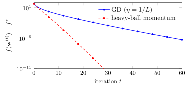\] For a strongly convex quadratic $f$, this iteration converges faster than plain GD (Polyak, 1987). Fig. 3 compares plain GD and heavy-ball momentum on a strongly convex quadratic function.

References

1. Goodfellow et al. (2016). Deep Learning. MIT Press.
2. Boyd and Vandenberghe (2004). Convex Optimization. Cambridge Univ. Press.
3. Helmke and Moore (1994). Optimization and Dynamical Systems. Springer.
4. Bauschke and Combettes (2011). Convex Analysis and Monotone Operator Theory in Hilbert Spaces. Springer Science+Business Media.
5. Nesterov (2004). Introductory Lectures on Convex Optimization: A Basic Course. Kluwer Academic.
6. Beck (2017). First-Order Methods in Optimization. SIAM-Society for Industrial and Applied Mathematics.
7. Bubeck (2015). Convex Optimization: Algorithms and Complexity. Found. Trends Mach. Learn..
8. Polyak (1987). Introduction to optimization. Optimization Software, Inc., Publications Division, New York.
9. Beck and Teboulle (2009). A fast iterative shrinkage-thresholding algorithm for linear inverse problems. SIAM J. Imaging Sci..

Cite this entry

@misc{dictml_gd,
  author = {Jung, Alexander},
  title = {gradient descent},
  howpublished = {Dictionary of Applied Machine Learning (course edition)},
  year = {2026},
  doi = {10.5281/zenodo.21569296},
  note = {ISBN 978-952-64-3013-3, CC BY 4.0, retrieved 2026-08-06},
  url = {https://dictionaryofml.org/terms/gd.html}
}