Python demo — a script that recomputes what this entry states and prints one line per check
A matrix is a rectangular array of numbers arranged in
rows and columns, the two-dimensional special case of an
array. The entry $A_{\sampleidx,\featureidx}$ of a
matrix $\mA \in \reals^{\samplesize \times \nrfeatures}$ sits
in row $\sampleidx$ and column $\featureidx$. A prominent
example in machine learning (ML) is the feature matrix of a dataset,
obtained by stacking the feature vectors of $\samplesize$
data points row-wise. A matrix represents several distinct
mathematical objects: a system of linear equations, such as the
normal equations of linear regression; a linear map
between two vector spaces, after fixing a basis for
each; or a tabular dataset with one row per
data point and one column per feature.
Definition
P-featuremtxConsider a spreadsheet of daily weather
records at one station: each row holds a single day, each column
one measurement such as temperature or humidity. Such a tabular
dataset holds $\samplesize$ data points, each described
by $\nrfeatures$ numerical features. The features of
the $\sampleidx$-th data point are collected in its
feature vector
$\featurevec^{(\sampleidx)} = \big(\feature^{(\sampleidx)}_{1},
\ldots, \feature^{(\sampleidx)}_{\nrfeatures}\big)^{\top} \in
\reals^{\nrfeatures}$, one entry per column of the spreadsheet.
Stacking these $\samplesize$ feature vectors row-wise, so that
the $\sampleidx$-th row is
$\big(\featurevec^{(\sampleidx)}\big)^{\top}$, produces an
$\samplesize \times \nrfeatures$ rectangular array of numbers. Its
entry in row $\sampleidx$ and column $\featureidx$ is the
$\featureidx$-th feature of the $\sampleidx$-th
data point. This two-dimensional numeric array is
referred to as the feature matrix $\featuremtx$ of the
dataset; Fig. 1 carries out the
construction on three days of the weather example.
Figure 1: A tabular dataset of $\samplesize = 3$
data points and the feature matrix built from it. Each
row of the table is one day, whose $\nrfeatures = 3$
measurements, temperature (temp.), humidity (humid.), and
pressure (press.), form the feature vector
$\featurevec^{(\sampleidx)} \in \reals^{3}$; the day column
indexes the data points and is not itself a feature,
so it does not appear in $\featuremtx$. Stacking
$\featurevec^{(1)}, \featurevec^{(2)}, \featurevec^{(3)}$ as rows
makes the entry $X_{\sampleidx,\featureidx}$ the $\featureidx$-th
measurement taken on day $\sampleidx$: $X_{2,3} = 1008$ is the
pressure on day $2$
More generally, a matrix of size $\samplesize \times \nrfeatures$
is a two-dimensional array of numbers denoted by
\[
\mA = \begin{pmatrix}
A_{1,1} & A_{1,2} & \dots & A_{1,\nrfeatures} \\
A_{2,1} & A_{2,2} & \dots & A_{2,\nrfeatures} \\
\vdots & \vdots & \ddots & \vdots \\
A_{\samplesize,1} & A_{\samplesize,2} & \dots & A_{\samplesize,\nrfeatures}
\end{pmatrix} \in \reals^{\samplesize \times \nrfeatures}\text{.}
\]
Here, $A_{\sampleidx,\featureidx}$ denotes the matrix entry
in the $\sampleidx$-th row and the $\featureidx$-th column.
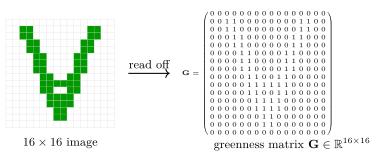
A digital image is a matrix of exactly this
kind. Recording how green each pixel is turns a $16 \times 16$ image
into a $16 \times 16$ matrix whose two indices are pixel positions
(Fig. 2).
Figure 2: A $16 \times 16$ pixel image of the "for all" quantifier
$\forall$ and the matrix of its green channel. Pixel
$(\sampleidx,\featureidx)$ has greenness $G_{\sampleidx,
\featureidx} = 1$ where the glyph is drawn and $0$ elsewhere, so
the $1$s trace the same shape in $\mG$ that the shaded squares
trace in the image
Matrices represent several distinct mathematical objects
(Strang, 2016), including the following:
Systems of linear equations: A matrix collects the
coefficients of a system of linear equations,
\[ \begin{pmatrix}
A_{1,1} & A_{1,2} \\
A_{2,1} & A_{2,2}
\end{pmatrix}
\begin{pmatrix}
x_1 \\
x_2
\end{pmatrix}
=\begin{pmatrix}
b_1 \\
b_2
\end{pmatrix}
\text{, written compactly as } \mA \vx = \vb \text{.}
\]
One important example is the normal equations
$\featuremtx^{\top}\featuremtx\,\weights = \featuremtx^{\top}\labelvec$,
whose solutions are the model parameters that minimize the
training error in linear regression.
Linear maps:
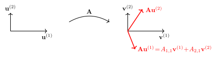
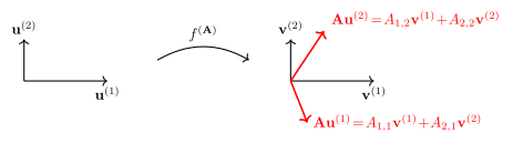
Consider two vector spaces $\mathcal{U}$ and $\vecspace$, of dimension $\nrfeatures$ and $\samplesize$, respectively.
Fixing a basis $\vu^{(1)},\,\ldots,\,\vu^{(\nrfeatures)}$ for $\mathcal{U}$ and a basis $\vv^{(1)},\,\ldots,\,\vv^{(\samplesize)}$
for $\vecspace$, each matrix $\mA \in \reals^{\samplesize \times \nrfeatures}$ defines a
linear map $f^{(\mA)}: \mathcal{U} \rightarrow \vecspace$ (see Fig. 3) via
\[f^{(\mA)}\big(\vu^{(\featureidx)}\big) = \sum_{\sampleidx=1}^{\samplesize} A_{\sampleidx,\featureidx} \vv^{(\sampleidx)}\text{.}\]
Taking $\mathcal{U} = \reals^{\nrfeatures}$ and
$\vecspace = \reals^{\samplesize}$ with the standard bases,
the image of a vector $\vx$ under $f^{(\mA)}$ is the
matrix-vector product $f^{(\mA)}(\vx) = \mA\vx$.
Datasets: As in the opening example, a matrix
can represent a dataset with each row holding a
single data point and each column a specific
feature or label.
Figure 3: The matrix $\mA$ defines a linear map $f^{(\mA)}$ between two
vector spaces: the basis vector $\vu^{(\featureidx)}$
is mapped to the vector (thick red arrows) whose
coordinates form the
$\featureidx$-th column of $\mA$
Written with the feature matrix, the
training error that empirical risk minimization (ERM)-based linear regression minimizes
becomes a succinct algebraic expression. Collecting the labels of the
training set in $\labelvec \in \reals^{\samplesize}$, the
training error of the hypothesis
$\hypothesis^{(\weights)}(\featurevec) \defeq \weights^{\top}\featurevec$
is
\[
(1/\samplesize)\,\normgeneric{\featuremtx \weights - \labelvec}{2}^{2}
\text{,}
\]
with gradient
$(2/\samplesize)\,\featuremtx^{\top}(\featuremtx \weights - \labelvec)$.
Each gradient descent (GD) step is therefore one multiplication by $\featuremtx$
followed by one by $\featuremtx^{\top}$, and equating the
gradient to zero leads back to the normal equations
from the first example above.
Matrices recur across machine learning (ML) beyond the feature matrix. The
Jacobian matrix and the Hessian collect the first- and
second-order partial derivatives of a multivariate
function and drive gradient-based training. The
covariance matrix records the pairwise covariances of a
probability distribution over features. Principal component analysis (PCA), singular value decomposition (SVD), and a
random projection factor or compress the feature matrix to
lower its dimension. A kernel method replaces explicit
feature vectors by a matrix of pairwise inner products, and
a tabular Markov decision process (MDP) stores its transition probabilities as a matrix.
A graph is carried by matrices as well: its
adjacency matrix records which nodes are joined and with what
edge weight, and the Laplacian matrix assembled from those weights is
the matrix whose eigenvectors graph clustering uses
to split the nodes into clusters (Luxburg, 2007).
See also: linear map, dataset, linear model,
vector, feature matrix, normal equations,
array, transpose.
References
Strang (2016). Introduction to Linear Algebra. Wellesley-Cambridge Press.