P-array writes when the script runsDictionary of Applied Machine Learning · matrix
Numerical companion to the entry matrix: it recomputes what the entry states and prints one line per check
One block per paragraph of the entry (marked [P...]): each block verifies numerically what the corresponding statement asserts. Self-contained (numpy/matplotlib only), fixed seed.
Run it without installing anything:uv run https://dictionaryofml.org/terms/matrix.py
uv downloads this script and the pinned NumPy and Matplotlib it needs, then runs it; the script fetches any input file it uses. To keep the output files, download matrix.py into a folder and run uv run matrix.py there. With NumPy and Matplotlib already installed, python3 matrix.py, from any directory — it writes its output files into the current directory. Fixed seeds, so the printed numbers reproduce exactly. Download matrix.py · Notebook · Open in Colab
One cell per block of the script: the code, and what that code printed when it last ran here
"""
matrix.py — numerical companion to the glossary entry 'matrix'.

One block per paragraph of the entry (marked [P...]): each block verifies
numerically what the corresponding statement asserts. Self-contained
(numpy/matplotlib only), fixed seed.

Blocks
------
[P-featuremtx] Stacking the feature vectors of m data points row-wise
               yields the m x d feature matrix: row r of X is x^(r) and
               entry X[r, j] is feature j of data point r.
[P-linsys]     A matrix represents a system of linear equations A w = y;
               the normal equations X^T X w = X^T y of least-squares
               linear regression are one instance — their solution
               matches the least-squares fit.
[P-linearmap]  A matrix defines a linear map: the image of basis vector
               u^(j) is the linear combination sum_r A[r, j] v^(r) of the
               target basis, and the map is additive and homogeneous.
[P-array]      A matrix is the order-2 special case of an array: its
               numpy representation has exactly two axes, while a scalar,
               a vector, an image, and a stack of images have order
               0, 1, 3, and 4.

Outputs
-------
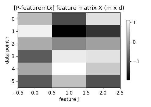
matrix.png : preview figure (checking only).

Data generated by pythondemos/matrix.py.
"""

import numpy as np
import matplotlib

matplotlib.use("Agg")
import matplotlib.pyplot as plt
from pathlib import Path

OUT_DIR = Path(__file__).parent

rng = np.random.default_rng(42)
report = []


def check(name, ok):
    report.append((name, bool(ok)))
    print(f"  [{'ok' if ok else 'FAIL'}] {name}")
Stacking the feature vectors of m data points row-wise yields the m x d feature matrix: row r of X is x^(r) and entry X[r, j] is feature j of data point r.
print("[P-featuremtx] feature matrix stacks feature vectors row-wise")
m, d = 6, 3
feature_vecs = [rng.normal(size=d) for _ in range(m)]
X = np.stack(feature_vecs, axis=0)
check("shape is m x d", X.shape == (m, d))
check("row r equals x^(r)",
      all(np.array_equal(X[r], feature_vecs[r]) for r in range(m)))
check("entry X[r, j] is feature j of data point r",
      X[2, 1] == feature_vecs[2][1])
# the printed A_{i,j} convention: entry in row i, column j
A_conv = np.array([[10 * i + j for j in range(1, 4)] for i in range(1, 3)])
check("A[i, j] sits in row i and column j (A_{1,2} = 12, A_{2,3} = 23)",
      A_conv[0, 1] == 12 and A_conv[1, 2] == 23)
[P-featuremtx] feature matrix stacks feature vectors row-wise
  [ok] shape is m x d
  [ok] row r equals x^(r)
  [ok] entry X[r, j] is feature j of data point r
  [ok] A[i, j] sits in row i and column j (A_{1,2} = 12, A_{2,3} = 23)
A matrix represents a system of linear equations A w = y; the normal equations X^T X w = X^T y of least-squares linear regression are one instance — their solution matches the least-squares fit.
print("[P-linsys] matrices represent linear systems (normal equations)")
y = X @ np.array([1.0, -2.0, 0.5]) + 0.1 * rng.normal(size=m)
w = np.linalg.solve(X.T @ X, X.T @ y)          # normal equations
w_lstsq = np.linalg.lstsq(X, y, rcond=None)[0]
check("normal-equation solution equals the least-squares fit",
      np.allclose(w, w_lstsq))
check("residual satisfies X^T (y - X w) = 0",
      np.max(np.abs(X.T @ (y - X @ w))) < 1e-10)
[P-linsys] matrices represent linear systems (normal equations)
  [ok] normal-equation solution equals the least-squares fit
  [ok] residual satisfies X^T (y - X w) = 0
A matrix defines a linear map: the image of basis vector u^(j) is the linear combination sum_r A[r, j] v^(r) of the target basis, and the map is additive and homogeneous.
print("[P-linearmap] a matrix defines a linear map")
A = rng.normal(size=(4, 3))
U = np.eye(3)                                   # basis of the domain
Vb = np.eye(4)                                  # basis of the codomain
for j in range(3):
    img = A @ U[:, j]
    combo = sum(A[r, j] * Vb[:, r] for r in range(4))
    check(f"image of u^({j+1}) is sum_r A[r,{j+1}] v^(r)",
          np.allclose(img, combo))
u1, u2, a = rng.normal(size=3), rng.normal(size=3), 2.7
check("additivity: A(u + u') = A u + A u'",
      np.allclose(A @ (u1 + u2), A @ u1 + A @ u2))
check("homogeneity: A(a u) = a A u", np.allclose(A @ (a * u1), a * (A @ u1)))
[P-linearmap] a matrix defines a linear map
  [ok] image of u^(1) is sum_r A[r,1] v^(r)
  [ok] image of u^(2) is sum_r A[r,2] v^(r)
  [ok] image of u^(3) is sum_r A[r,3] v^(r)
  [ok] additivity: A(u + u') = A u + A u'
  [ok] homogeneity: A(a u) = a A u
A matrix is the order-2 special case of an array: its numpy representation has exactly two axes, while a scalar, a vector, an image, and a stack of images have order 0, 1, 3, and 4.
print("[P-array] a matrix is an order-2 array")
scalar = np.float64(3.0)
vector = rng.normal(size=5)
image = rng.normal(size=(32, 32, 3))            # H x W x C
batch = rng.normal(size=(8, 32, 32, 3))         # a stack of 8 images
check("matrix has exactly two axes", X.ndim == 2)
check("scalar / vector / image / image stack have order 0 / 1 / 3 / 4",
      (scalar.ndim, vector.ndim, image.ndim, batch.ndim) == (0, 1, 3, 4))

# ------------------------------------------------------------ preview
fig, ax = plt.subplots(figsize=(4.5, 3.2))
im = ax.imshow(X, cmap="gray", aspect="auto")
ax.set_xlabel("feature j"); ax.set_ylabel("data point r")
ax.set_title("[P-featuremtx] feature matrix X (m x d)")
fig.colorbar(im, ax=ax, shrink=0.8)
fig.tight_layout()
fig.savefig(OUT_DIR / "matrix.png", dpi=110)
print(f"\n{sum(ok for _, ok in report)}/{len(report)} checks passed")
assert all(ok for _, ok in report)
[P-array] a matrix is an order-2 array
  [ok] matrix has exactly two axes
  [ok] scalar / vector / image / image stack have order 0 / 1 / 3 / 4

13/13 checks passed
P-array writes when the script runs