empirical risk minimization

Machine learning (ML) methods aim to find a hypothesis that yields accurate predictions, reflected by a small loss. Empirical risk minimization (ERM) formalizes this: it selects a hypothesis with minimal empirical risk, i.e., minimal average loss on a training set $\trainset$. Different ML methods arise from different choices of the model $\hypospace$ and the loss function $\lossfun$, both of which depend on the feature space $\featurespace$ and the label space $\labelspace$ of a given method. The entry also covers the online form of ERM (Follow-The-Leader (FTL)) and contrasts ERM with reinforcement learning (RL) methods that use a different access mechanism for the loss values.

Definition

A weather forecaster predicting tomorrow's maximum daytime temperature is useful only if its predictions are accurate on most days. This forecaster is a hypothesis: it maps a day's features to a prediction of tomorrow's temperature, and its loss quantifies how far that prediction lies from the measured value. More generally, machine learning (ML) methods aim to find a hypothesis that incurs a small loss for any data point. But what does any data point mean? One way to make this notion precise is to use a probabilistic model for the generation of data points.

If data points are assumed to be drawn from a probability distribution, then the risk of a hypothesis is defined as the expectation of its loss under that probability distribution. The ideal choice is then the hypothesis with minimal risk. However, in most ML applications, the underlying probability distribution is not known. Instead, only a finite training set $\trainset$ of data points is available. ERM replaces the intractable risk with its sample-average surrogate, the empirical risk on $\trainset$, and picks the hypothesis that minimizes this surrogate (Hastie et al., 2009; Murphy, 2012; Shalev-Shwartz and Ben-David, 2014; Vapnik, 2000).

For a fixed choice of loss function and hypothesis space, ERM is a map $\algomap$ that reads in a training set $\trainset = \{\datapoint^{(\sampleidx)}\}_{\sampleidx=1}^{\samplesize}$ of data points $\datapoint^{(\sampleidx)} = \pair{\featurevec^{(\sampleidx)}}{\truelabel^{(\sampleidx)}}$ and returns a learned hypothesis $\learnthypothesis = \algomap(\trainset) \in \hypospace$ that minimizes the empirical risk on $\trainset$, \[ \learnthypothesis \in \argmin_{\hypothesis \in \hypospace} \frac{1}{\samplesize} \sum_{\sampleidx=1}^{\samplesize} \lossfunc{\datapoint^{(\sampleidx)}}{\hypothesis} \text{.} \] The hypothesis $\learnthypothesis$ is chosen from the underlying hypothesis space (or model) $\hypospace$. For an ERM-based method, model training is to compute $\algomap$.

In practice, the map $\algomap$ is computed by an iterative optimization method. Many of these optimization methods can be represented as a fixed-point iteration that starts with an initial hypothesis $\hypothesis^{(0)}$ and then repeatedly applies an update operator $\fixedpointop$, \[\hypothesis^{(\iteridx+1)} = \fixedpointop\big( \hypothesis^{(\iteridx)} \big) \text{, for } \iteridx=0,1,\ldots \text{.}\] The update operator $\fixedpointop$ depends on the training set, the loss function, and the hypothesis space. It is chosen such that its fixed points are minimizers of the empirical risk.

For ERM using a parametric model $\hypospace$, the fixed-point iteration can be formulated directly in terms of the model parameters $\weights$ instead of the hypothesis $\hypothesis$. In particular, starting with initial model parameters $\weights^{(0)}$, the update operator $\fixedpointop$ is applied repeatedly to the model parameters, \[\weights^{(\iteridx+1)} = \fixedpointop\big( \weights^{(\iteridx)} \big) \text{, for } \iteridx=0,1,\ldots \text{.}\] One important example of such a fixed-point iteration is gradient descent (GD), which updates the model parameters in the direction of the negative gradient of the empirical risk (which needs to be differentiable).

ERM presupposes that the loss $\lossfunc{\datapoint^{(\sampleidx)}}{\hypothesis}$ can be evaluated for every hypothesis $\hypothesis \in \hypospace$ and every training data point $\datapoint^{(\sampleidx)}$. This full-feedback requirement is what distinguishes ERM from reinforcement learning (RL) algorithms, which use partial feedback. In particular, at each time instant $\timeidx$, an RL algorithm chooses a hypothesis $\learnthypothesis^{(\timeidx)}$ delivering a prediction (or action) and only measures the loss incurred by this hypothesis. It has no information about the loss that would have been incurred by any other hypothesis $\hypothesis \in \hypospace \setminus \{\learnthypothesis^{(\timeidx)}\}$.

ERM can also be implemented as an online algorithm, which is useful when the data points in $\trainset$ can only be accessed sequentially. Such sequential access arises, for instance, when memory limits prevent loading the entire training set at once. The canonical online form of ERM is the Follow-The-Leader (FTL) algorithm, which, at every round, solves a partial ERM problem on all data points seen so far. Assuming that the data point $\datapoint^{(\timeidx)}$ arrives at time instant $\timeidx=1,2,\ldots$, FTL updates the learned hypothesis $\learnthypothesis^{(\timeidx)}$ by \[ \learnthypothesis^{(\timeidx)} \in \argmin_{\hypothesis \in \hypospace} \frac{1}{\timeidx} \sum_{\sampleidx=1}^{\timeidx} \lossfunc{\datapoint^{(\sampleidx)}}{\hypothesis} \text{.}\] Implementing this partial ERM separately for each time instant can become computationally expensive (and wasteful), as it does not exploit the similarity between consecutive partial ERM problems. This similarity can be exploited by online gradient descent (online GD), which performs a single GD step on the new data point $\datapoint^{(\timeidx)}$ at every time instant $\timeidx$ (Hazan, 2022, Sect. 3.1).

Different ML methods arise from different design choices for the two ingredients of the map $\algomap$: the model $\hypospace$ and the loss function $\lossfun$ (Jung, 2022, Ch. 3). Both depend on the nature of the data points, i.e., on the feature space $\featurespace$ and the label space $\labelspace$. For example, image data points with a high-dimensional feature space and a finite label space typically call for an artificial neural network (ANN) together with the logistic loss. Conversely, data points with few real-valued features and a real-valued label often allow for a linear model together with the squared error loss.

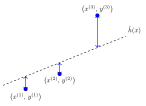
Fig. 1 illustrates ERM for a linear model on data points with a single feature $\feature$ and label $\truelabel$. Each hypothesis is a linear map $\hypothesis(\feature) = \weight_{1} \feature + \weight_{0}$ with model parameters $\weight_{0}, \weight_{1}$. ERM picks the model parameters that minimize the empirical risk on $\trainset$.

See also: optimization problem, loss, loss function, empirical risk, risk, training set, hypothesis space, model, hypothesis, algorithm, training, generalization, optimization method, gradient descent, online algorithm, online gradient descent, Follow-The-Leader, reinforcement learning.

Definition

References

Cite this entry