P-fixedpoint writes when the script runsDictionary of Applied Machine Learning · empirical risk minimization (ERM)
Numerical companion to the entry empirical risk minimization (ERM): it recomputes what the entry states and prints one line per check
One block per paragraph of the entry (marked [P...]): each block verifies numerically what the corresponding statement asserts. Self-contained (numpy/matplotlib only), fixed seed.
Run it without installing anything:uv run https://dictionaryofml.org/terms/erm.py
uv downloads this script and the pinned NumPy and Matplotlib it needs, then runs it; the script fetches any input file it uses. To keep the output files, download erm.py into a folder and run uv run erm.py there. With NumPy and Matplotlib already installed, python3 erm.py, from any directory — it writes its output files into the current directory. Fixed seeds, so the printed numbers reproduce exactly. Download erm.py · Notebook · Open in Colab
One cell per block of the script: the code, and what that code printed when it last ran here
"""
erm.py — numerical companion to the glossary entry
'empirical risk minimization (ERM)'.

One block per paragraph of the entry (marked [P...]): each block verifies
numerically what the corresponding statement asserts. Self-contained
(numpy/matplotlib only), fixed seed.

Blocks
------
[P-risk]       The risk of a hypothesis is the expected loss under the
               data-generating distribution; the ideal choice minimizes
               the risk (verified on a grid of hypotheses against a
               large Monte Carlo sample).
[P-surrogate]  The distribution is unknown; ERM minimizes the
               sample-average surrogate. As the trainset grows, the
               risk of the ERM hypothesis approaches the minimal risk
               (consistency of the surrogate).
[P-map]        ERM is a map A: trainset -> learned hypothesis. For
               the linear model with squared error loss the map has a closed
               form, its output attains the minimal empirical risk, and
               calling it on different trainsets yields different
               learned hypotheses.
[P-fixedpoint] In practice A is computed by an iterative optimization
               method that is a fixed-point iteration: the GD update
               operator T has the ERM solution as its fixed point
               (T(w-hat) = w-hat), and iterating T converges to it.

Outputs
-------
erm.png : preview figure (checking only).

Data generated by pythondemos/erm.py.
"""

import numpy as np
import matplotlib

matplotlib.use("Agg")
import matplotlib.pyplot as plt
from pathlib import Path

OUT_DIR = Path(__file__).parent

rng = np.random.default_rng(42)
report = []


def check(name, ok):
    report.append((name, bool(ok)))
    print(f"  [{'ok' if ok else 'FAIL'}] {name}")


# data-generating distribution: y = 2 x + 1 + noise, x ~ U(0, 10)
W_TRUE = np.array([2.0, 1.0])
def draw(m):
    x = rng.uniform(0, 10, m)
    y = W_TRUE[0] * x + W_TRUE[1] + 0.5 * rng.normal(size=m)
    return x, y

def risk(w, mc=200000):                            # expected squared loss
    x, y = draw(mc)
    return np.mean((y - w[0] * x - w[1]) ** 2)
The risk of a hypothesis is the expected loss under the data-generating distribution; the ideal choice minimizes the risk (verified on a grid of hypotheses against a large Monte Carlo sample).
print("[P-risk] risk = expected loss; the ideal hypothesis minimizes it")
cands = [np.array([a, b]) for a in (1.5, 2.0, 2.5) for b in (0.0, 1.0)]
risks = [risk(w) for w in cands]
best = cands[int(np.argmin(risks))]
check("the risk-minimizing candidate is the true hypothesis (2, 1)",
      np.array_equal(best, W_TRUE))
check("its risk equals the noise floor 0.25 (irreducible)",
      abs(min(risks) - 0.25) < 0.01)
[P-risk] risk = expected loss; the ideal hypothesis minimizes it
  [ok] the risk-minimizing candidate is the true hypothesis (2, 1)
  [ok] its risk equals the noise floor 0.25 (irreducible)
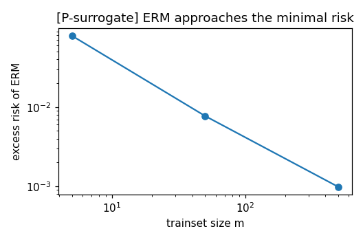
The distribution is unknown; ERM minimizes the sample-average surrogate. As the trainset grows, the risk of the ERM hypothesis approaches the minimal risk (consistency of the surrogate).
print("[P-surrogate] ERM minimizes the sample-average surrogate")
def erm_fit(m):
    x, y = draw(m)
    return np.polyfit(x, y, 1)
excess = [np.mean([risk(erm_fit(m)) - 0.25 for _ in range(20)])
          for m in (5, 50, 500)]
print(f"    excess risk of ERM at m = 5, 50, 500: "
      f"{excess[0]:.4f}, {excess[1]:.4f}, {excess[2]:.5f}")
check("the ERM hypothesis approaches the minimal risk as m grows",
      excess[0] > excess[1] > excess[2] > 0)
[P-surrogate] ERM minimizes the sample-average surrogate
    excess risk of ERM at m = 5, 50, 500: 0.0791, 0.0077, 0.00099
  [ok] the ERM hypothesis approaches the minimal risk as m grows
ERM is a map A: trainset -> learned hypothesis. For the linear model with squared error loss the map has a closed form, its output attains the minimal empirical risk, and calling it on different trainsets yields different learned hypotheses.
print("[P-map] ERM is a map from trainsets to hypotheses")
x1, y1 = draw(30)
x2, y2 = draw(30)
A = lambda x, y: np.polyfit(x, y, 1)
w1, w2 = A(x1, y1), A(x2, y2)
emp = lambda w, x, y: np.mean((y - w[0] * x - w[1]) ** 2)
check("A(D) attains the minimal empirical risk on D (vs perturbations)",
      all(emp(w1 + d, x1, y1) > emp(w1, x1, y1)
          for d in ([0.05, 0], [-0.05, 0], [0, 0.2], [0, -0.2])))
check("different trainsets yield different learned hypotheses",
      not np.allclose(w1, w2))
[P-map] ERM is a map from trainsets to hypotheses
  [ok] A(D) attains the minimal empirical risk on D (vs perturbations)
  [ok] different trainsets yield different learned hypotheses
In practice A is computed by an iterative optimization method that is a fixed-point iteration: the GD update operator T has the ERM solution as its fixed point (T(w-hat) = w-hat), and iterating T converges to it.
print("[P-fixedpoint] the optimizer is a fixed-point iteration")
X = np.c_[x1, np.ones(30)]
w_hat = np.linalg.solve(X.T @ X, X.T @ y1)         # ERM solution
L = 2 * np.linalg.eigvalsh(X.T @ X / 30).max()
T = lambda w: w - (1 / L) * (2 / 30) * X.T @ (X @ w - y1)   # GD operator
check("the ERM solution is a fixed point: T(w-hat) = w-hat",
      np.allclose(T(w_hat), w_hat, atol=1e-10))
w = np.zeros(2)
for _ in range(60000):     # ill-conditioned (x vs intercept): slow rate
    w = T(w)
check("iterating T converges to the ERM solution",
      np.linalg.norm(w - w_hat) < 1e-5)

# ------------------------------------------------------------ preview
fig, ax = plt.subplots(figsize=(4.8, 3.2))
ax.loglog([5, 50, 500], excess, "o-")
ax.set_xlabel("trainset size m"); ax.set_ylabel("excess risk of ERM")
ax.set_title("[P-surrogate] ERM approaches the minimal risk")
fig.tight_layout()
fig.savefig(OUT_DIR / "erm.png", dpi=110)
print(f"\n{sum(ok for _, ok in report)}/{len(report)} checks passed")
assert all(ok for _, ok in report)
[P-fixedpoint] the optimizer is a fixed-point iteration
  [ok] the ERM solution is a fixed point: T(w-hat) = w-hat
  [ok] iterating T converges to the ERM solution

7/7 checks passed
P-fixedpoint writes when the script runs