Dictionary of Applied Machine Learning
Updated on 2026-09-17
Typeset PDF version — the authoritative form of this entry
Python demo — a script that recomputes what this entry states and prints one line per check
Linear regression is a regression method that learns a linear hypothesis map for predicting the numeric label of a data point from its features. Its least squares variant chooses a map that minimizes the average squared error loss on a training set. Linear regression is an instance of empirical risk minimization (ERM) that is obtained by using the linear model and the squared error loss. The optimal model parameters are determined by the normal equations. This system can be solved in closed form or iteratively, for example, by gradient descent (GD). Adding a penalty term to the average squared error loss yields regularized variants such as ridge regression and least absolute shrinkage and selection operator (Lasso).
P1/P2Linear regression methods learn a linear hypothesis map that delivers a prediction of the numeric label of a data point. The prediction is based solely on the features of the data point, which are fed as input to the learned hypothesis map. Linear regression can be used to predict tomorrow's temperature from weather measurements recorded over the last five days, using them as features and tomorrow's temperature as the label (Jung, 2022, Sect. 2.1).
P1/P2Formally, linear regression learns a linear hypothesis map $\hypothesis^{(\weights)}(\featurevec) = \weights^{\top}\featurevec$ to predict the numeric label $\truelabel \in \reals$ of a data point from its feature vector $\featurevec = \big(\feature_{1},\,\ldots,\,\feature_{\nrfeatures}\big)^{\top} \in \reals^{\nrfeatures}$. Here, $\nrfeatures$ denotes the number of features of a data point. The model parameters $\weights$ are learned from a training set $\trainset = \big\{ \pair{\featurevec^{(\sampleidx)}}{\truelabel^{(\sampleidx)}} \big\}_{\sampleidx=1}^{\samplesize}$ of data points. Appending a constant feature to $\featurevec$ lets one entry of $\weights$ act as an intercept, so $\weights^{\top}\featurevec$ represents an affine function of the original measurements. In what follows, $\featurevec$ denotes the feature vector that is fed to the linear hypothesis map. It can be either the original or the augmented feature vector.
P3The least squares variant of linear regression measures the quality of a
linear hypothesis map by the average squared error loss on the
training set. As an instance of empirical risk minimization (ERM), it learns the
model parameters $\weights$ by solving the optimization problem
\[
\min_{\weights \in \reals^{\nrfeatures}} \frac{1}{\samplesize}
\sum_{\sampleidx=1}^{\samplesize}
\big( \truelabel^{(\sampleidx)} - \weights^{\top} \featurevec^{(\sampleidx)} \big)^{2} \text{.}
\]
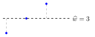
Fig. 1 illustrates this linear regression problem
for a training set with a constant scalar feature $\feature^{(\sampleidx)}=1$
for $\sampleidx=1,\ldots,\samplesize$.
P4-P6However, the solution of the normal equations \(\eqref{eq_linreg_normal_eq_dict}\) is unique only if the feature matrix $\featuremtx$ has full column rank. This requires at least as many data points as features, $\samplesize \geq \nrfeatures$. When this holds, and the columns of $\featuremtx$ are linearly independent, the matrix $\featuremtx^{\top}\featuremtx$ is invertible and the normal equations \(\eqref{eq_linreg_normal_eq_dict}\) have the unique closed-form solution $\widehat{\weights} = \big(\featuremtx^{\top}\featuremtx\big)^{-1} \featuremtx^{\top} \labelvec$.
P4-P6If instead $\samplesize < \nrfeatures$ (more features than data points), $\featuremtx$ cannot have full column rank, $\featuremtx^{\top}\featuremtx$ is singular, and the optimization problem has infinitely many solutions. All of them incur the same minimal average squared error loss on the training set, but their predictions for data points outside the training set can differ arbitrarily. Choosing among them is therefore a matter of generalization (see overfitting). A unique solution can be selected, for example, by picking the minimum-norm solution $\pinv{\featuremtx} \labelvec$ given by the pseudoinverse $\pinv{\featuremtx}$. A common remedy is regularization: adding a penalty term to the average squared error loss. The penalty term can be interpreted as an estimate of how much higher the loss is on data points outside the training set than on it (Hastie et al., 2009, Ch. 7). This yields regularized variants of linear regression, with ridge regression using the penalty term $\regparam \normgeneric{\weights}{2}^{2}$ and the least absolute shrinkage and selection operator (Lasso) using the penalty term $\regparam \normgeneric{\weights}{1}$.
P4-P6Linear regression also has a statistical interpretation. Consider a probabilistic model with a joint probability distribution $\probdist^{(\featurevec, \truelabel)}$ over the features and the label. Under the squared error loss, the Bayes estimator (i.e., the hypothesis with minimum risk) is the conditional expectation $\expect\{\truelabel \mid \featurevec\}$ (Lehmann and Casella, 1998, Ch. 4; Papoulis and Pillai, 2002). In this statistical interpretation, $\featurevec$ denotes the original feature vector. When the features and the label are jointly Gaussian random variables (Gaussian RVs) with zero mean and invertible covariance matrix $\covmtx{\featurevec} = \expect\{\featurevec\featurevec^{\top}\}$, this Bayes estimator is \[ \bayeshypothesis(\featurevec) = \big(\weights^{\star}\big)^{\top}\featurevec \text{, with } \weights^{\star} = \big(\covmtx{\featurevec}\big)^{-1}\, \covvec{\featurevec,\truelabel} \text{.} \] Here, $\covvec{\featurevec,\truelabel} = \expect\{\featurevec\truelabel\}$ is the covariance between the features $\featurevec$ and the label $\truelabel$. This Bayes estimator is linear in $\featurevec$. Without the zero-mean assumption, it is an affine function of $\featurevec$. However, as for the linear hypothesis map above, the intercept can be absorbed by appending a constant feature. Least-squares linear regression is the ERM counterpart of this predictor: it replaces $\covmtx{\featurevec}$ and $\covvec{\featurevec,\truelabel}$ with the sample-based estimates $(1/\samplesize)\featuremtx^{\top}\featuremtx$ and $(1/\samplesize)\featuremtx^{\top}\labelvec$, recovering, for invertible $\featuremtx^{\top}\featuremtx$, the unique solution $\widehat{\weights} = \big(\featuremtx^{\top}\featuremtx\big)^{-1}\featuremtx^{\top}\labelvec$ of the normal equations \(\eqref{eq_linreg_normal_eq_dict}\).
P7Instead of solving the normal equations \(\eqref{eq_linreg_normal_eq_dict}\) directly (via the inverse matrix or pseudoinverse), machine learning (ML) methods often solve it by an iterative optimization method, as implemented in widely used ML software libraries such as scikit-learn (Pedregosa et al., 2011) and PyTorch (Paszke et al., 2019). Starting from initial model parameters $\weights^{(0)}$, such a method repeatedly applies an update operator $\fixedpointop$, \[ \weights^{(\iteridx+1)} = \fixedpointop\big(\weights^{(\iteridx)}\big) \text{, for } \iteridx = 0,1,\ldots \text{.} \] The operator $\fixedpointop$ is designed such that the sequence of model parameters $\weights^{(\iteridx)}$ converges to a solution of the normal equations \(\eqref{eq_linreg_normal_eq_dict}\).
P8One important example of such an iterative optimization method is gradient descent (GD), which uses the GD step operator \[ \gdstep{\lrate}(\weights) = \weights - \lrate \nabla f(\weights) \text{.} \] Here, $\lrate > 0$ is a step size that must be chosen small enough to ensure convergence (Bertsekas, 2016, Sect. 1.2). The superscript in $\gdstep{\lrate}$ makes the dependence of the operator on $\lrate$ explicit. Inserting the average training error into the general form of the GD step yields the explicit update \[ \begin{aligned} \gdstep{\lrate}(\weights) &= \weights + \frac{2\lrate}{\samplesize} \sum_{\sampleidx=1}^{\samplesize} \big( \truelabel^{(\sampleidx)} - \weights^{\top}\featurevec^{(\sampleidx)} \big) \featurevec^{(\sampleidx)} \\ &= \Big(\mI - \frac{2\lrate}{\samplesize}\featuremtx^{\top}\featuremtx\Big)\weights + \frac{2\lrate}{\samplesize}\featuremtx^{\top}\labelvec \text{.} \end{aligned} \]
P9-P12The fixed points of $\gdstep{\lrate}$ are exactly the solutions of the normal equations \(\eqref{eq_linreg_normal_eq_dict}\), since $\gdstep{\lrate}(\widehat{\weights}) = \widehat{\weights}$ holds if and only if $\featuremtx^{\top}\featuremtx\widehat{\weights} = \featuremtx^{\top}\labelvec$. The update operator is affine, \[\gdstep{\lrate}(\weights) = \mM \weights + \vb \text{,}\] with linear part $\mM = \mI - (2\lrate/\samplesize)\featuremtx^{\top}\featuremtx$ and offset $\vb = (2\lrate/\samplesize)\, \featuremtx^{\top}\labelvec$.
P9-P12When $\featuremtx$ has full column rank, so that $\featuremtx^{\top}\featuremtx$ is positive definite, $\gdstep{\lrate}$ is a contractive operator with respect to the Euclidean norm for every step size $0 < \lrate < \samplesize/\eigval{\max}$. Here, $\eigval{\max}$ is the largest eigenvalue of $\featuremtx^{\top}\featuremtx$: the eigenvalues of the linear part $\mM$ are $1 - (2\lrate/\samplesize)\,\eigval{\featureidx}$, with the positive eigenvalues $\eigval{\featureidx}$ of $\featuremtx^{\top}\featuremtx$, and they lie strictly between $-1$ and $1$ exactly for such step sizes (cf. Nesterov, 2004, Thm. 2.1.14, which covers GD for any smooth, strongly convex objective function and step sizes $\lrate \leq \samplesize/(\eigval{\min} + \eigval{\max})$, with the smallest eigenvalue $\eigval{\min}$ of $\featuremtx^{\top}\featuremtx$). The fixed-point iteration converges to the unique solution $\widehat{\weights}$. Moreover, the convergence speed of GD is governed by the ratio of the largest to the smallest eigenvalue of $\featuremtx^{\top}\featuremtx$, that is, by its condition number $\condnumber{\featuremtx^{\top}\featuremtx} = \eigval{\max}/\eigval{\min}$ (Boyd and Vandenberghe, 2004, Sect. 9.3).
P9-P12The GD step above uses the entire training set to compute the gradient. When the data points instead arrive sequentially at time instants $\iteridx=1,2,\ldots$, or the training set is too large to fit in memory, the model parameters can be learned by online gradient descent (online GD). At each time step $\iteridx$, it applies a single GD step using only the arriving data point $\pair{\featurevec^{(\iteridx)}}{\truelabel^{(\iteridx)}}$, \[ \weights^{(\iteridx+1)} = \weights^{(\iteridx)} + 2\lrate \big( \truelabel^{(\iteridx)} - \big(\weights^{(\iteridx)}\big)^{\top} \featurevec^{(\iteridx)} \big) \featurevec^{(\iteridx)} \text{.} \] This is the GD step on the loss function $\big(\truelabel^{(\iteridx)} - \weights^{\top}\featurevec^{(\iteridx)}\big)^{2}$ of the arriving data point alone, rather than on the average squared error loss $f(\weights)$. It is the least mean squares (LMS) update (Bishop, 2006, Sect. 3.1.3). It avoids storing the entire training set, and its per-iteration complexity is independent of the training set size $\samplesize$.
P13The optimality condition \(\eqref{eq_linreg_normal_eq_dict}\) allows one to study the stability of linear regression. Ideally, the learned model parameters are insensitive to limited perturbations of the training set. A label-only perturbation, for example, replaces a single label of the training set with an outlier or another corrupted value. A perturbed training set yields a feature matrix $\widetilde{\featuremtx} = \featuremtx + \Delta \featuremtx$ and a label vector $\widetilde{\labelvec} = \labelvec + \Delta \labelvec$, with perturbation matrix $\Delta \featuremtx$ and vector $\Delta \labelvec$. This gives the perturbed normal equations \begin{equation} \label{eq_linreg_perturbed_normal_eq_dict} \widetilde{\featuremtx}^{\top} \widetilde{\featuremtx} \widetilde{\weights} = \widetilde{\featuremtx}^{\top} \widetilde{\labelvec} \text{.} \end{equation} Matrix perturbation theory quantifies how much $\widetilde{\weights}$ deviates from a solution $\widehat{\weights}$ of the clean normal equations \(\eqref{eq_linreg_normal_eq_dict}\) (Golub and Loan, 2013, Sect. 2.6).
P14For a label-only perturbation, $\Delta \featuremtx = \mathbf{0}$, the perturbed
and clean normal equations share the coefficient matrix
$\featuremtx^{\top}\featuremtx$. Assume $\featuremtx$ has full column rank,
so $\featuremtx^{\top}\featuremtx$ is invertible and the solution is unique.
Subtracting the clean normal equations \(\eqref{eq_linreg_normal_eq_dict}\)
from the perturbed normal equations \(\eqref{eq_linreg_perturbed_normal_eq_dict}\)
yields
\[
\widetilde{\weights} - \widehat{\weights} = \big(\featuremtx^{\top}\featuremtx\big)^{-1} \featuremtx^{\top} \Delta\labelvec = \pinv{\featuremtx} \Delta\labelvec \text{,}
\]
with the pseudoinverse $\pinv{\featuremtx}$. This in turn allows one to quantify the effect of
perturbing the training set as
\[
\normgeneric{\widetilde{\weights} - \widehat{\weights}}{2} \leq \normgeneric{\pinv{\featuremtx}}{2}\, \normgeneric{\Delta\labelvec}{2} \text{.}
\]
When $\featuremtx$ has full column rank,
$\normgeneric{\pinv{\featuremtx}}{2} = 1/\sqrt{\eigval{\min}(\featuremtx^{\top}\featuremtx)}
= \sqrt{\condnumber{\featuremtx^{\top}\featuremtx}}/\normgeneric{\featuremtx}{2}$,
where $\condnumber{\featuremtx^{\top}\featuremtx} = \eigval{\max}/\eigval{\min}$ is the condition number of $\featuremtx^{\top}\featuremtx$.
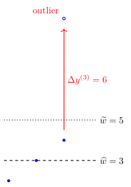
In the setting of Fig. 1, $\featuremtx = \mathbf{1}$ (the
all-ones vector), so $\pinv{\featuremtx} \Delta\labelvec =
(1/\samplesize) \sum_{\sampleidx=1}^{\samplesize} \Delta\truelabel^{(\sampleidx)}$.
Fig. 2 illustrates such a label-only
perturbation of the training set from Fig. 1:
the single label perturbation
$\Delta\truelabel^{(3)} = 6$ gives
$\widetilde{w} - \widehat{w} = 6/3 = 2$, i.e., the outlier pulls the
average of the labels upward, from
$\widehat{w} = 3$ to $\widetilde{w} = 5$.
See also: regression, linear model, least squares, empirical risk minimization, squared error loss, gradient descent, online gradient descent, online algorithm, ridge regression, least absolute shrinkage and selection operator, pseudoinverse, data point, feature, label, overfitting, Bayes estimator, risk, least mean squares, stochastic gradient descent.
@misc{dictml_linreg,
  author = {Jung, Alexander},
  editor = {Olioumtsevits, Konstantina and Schnoor, Ekkehard},
  title = {linear regression},
  howpublished = {Dictionary of Applied Machine Learning (course edition)},
  year = {2026},
  doi = {10.5281/zenodo.21569296},
  note = {ISBN 978-952-64-3013-3, CC BY 4.0, retrieved 2026-09-21},
  url = {https://dictionaryofml.org/terms/linreg.html}
}