Python demo — a script that recomputes what this entry states and prints one line per check
Regularization refers to modifications to a
machine learning (ML) method that improve its generalization.
Three routes are distinguished by which component of the
method is modified: pruning the hypothesis space, adding
a penalty term to the loss function, and augmenting
the training set with perturbed copies of its
data points. The three routes are often
interchangeable. As a case in point, applying
data augmentation to an empirical risk minimization (ERM)-based method is
equivalent to adding a penalty term to the training error.
P-routesFor ERM-based methods, regularization can be done in
three ways:
Model pruning: shrink the hypothesis space $\hypospace$ (the set of
candidate hypotheses $\hypothesis$) to a smaller $\hypospace'$. For a parametric model, the
shrinkage can be implemented via constraints on the
model parameters (e.g., $\weight_{1} \in [0.4,0.6]$
on the weight of feature
$\feature_{1}$ in linear regression).
Loss penalization: add a penalty term
to the training error of ERM. The penalty
estimates how much higher the risk is than
the average loss on the training set.
Data augmentation: enlarge the training set
$\trainset$ with perturbed copies of its
data points (e.g., adding the realizations of
independent and identically distributed (i.i.d.) random variables (RVs) to the feature vector of each data point).
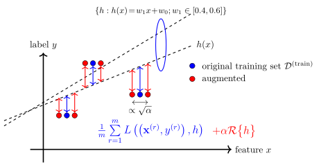
Fig. 1 illustrates the
three routes.
Figure 1: Three routes to regularization of an ERM-based method, shown for linear regression.
1) Model pruning: constraining the model parameters (here $\weight_{1} \in [0.4,0.6]$) shrinks the hypothesis space to the hypotheses inside the blue ellipse.
2) Loss penalization: the red penalty term $\regparam \regularizer{\hypothesis}$ is added to the blue training error near the bottom of the plot.
3) Data augmentation: the original data points (blue) are augmented with perturbed copies (red), displaced by an amount $\propto \sqrt{\regparam}$ (double arrow shown for the rightmost group)
These routes can yield the same learned
hypothesis. As an example, consider data augmentation for
linear regression that adds zero-mean perturbations with covariance matrix
$\sigma^{2} \mI$ to the feature vector of each
data point. Asymptotically in the number of perturbations,
the resulting learned hypothesis coincides with the one
obtained from ridge regression. Ridge regression adds
the penalty term $\sigma^{2} \normgeneric{\weights}{2}^{2}$
to the training error of linear regression
(Bishop, 1995;
Goodfellow et al., 2016, Sect. 7.5).
According to Lagrangian duality, adding this
penalty term is equivalent to shrinking the hypothesis space
to the set of hypotheses with
$\normgeneric{\weights}{2}^{2} \leq C$ for some constant $C$
(Bertsekas, 2016;
Hastie et al., 2009, Sect. 3.4.1).
P-equivThe above regularization techniques are not limited to
ERM-based methods but can also be applied to other
types of ML algorithms. For example, in online learning, the
Follow-The-Leader (FTL) method can be regularized by adding a
regularizer to the per-round
objective function of FTL. The resulting Follow-The-Regularized-Leader (FTRL) method
achieves lower regret than plain FTL
(Hazan, 2022, Ch. 5). Another
instance of regularization is the use of a prior distribution
over $\hypospace$ in Bayesian inference. The prior distribution
effectively acts as a regularizer by steering
the resulting posterior distribution (Bishop, 2006, Sect. 3.3).
See also:overfitting, generalization,
empirical risk minimization, model pruning, penalty term,
data augmentation, ridge regression, least absolute shrinkage and selection operator,
Follow-The-Regularized-Leader, prior distribution.
References
Goodfellow et al. (2016). Deep Learning. MIT Press.
Hastie et al. (2009). The Elements of Statistical Learning: Data Mining, Inference, and Prediction. Springer Science+Business Media. doi.org/10.1007/978-0-387-84858-7