P-equiv writes when the script runsDictionary of Applied Machine Learning · regularization
Numerical companion to the entry regularization: it recomputes what the entry states and prints one line per check
One block per paragraph of the entry (marked [P...]): each block verifies numerically what the corresponding statement asserts. Self-contained (numpy/matplotlib only), fixed seed.
Run it without installing anything:uv run https://dictionaryofml.org/terms/regularization.py
uv downloads this script and the pinned NumPy and Matplotlib it needs, then runs it; the script fetches any input file it uses. To keep the output files, download regularization.py into a folder and run uv run regularization.py there. With NumPy and Matplotlib already installed, python3 regularization.py, from any directory — it writes its output files into the current directory. Fixed seeds, so the printed numbers reproduce exactly. Download regularization.py · Notebook · Open in Colab
One cell per block of the script: the code, and what that code printed when it last ran here
"""
regularization.py — numerical companion to the glossary entry
'regularization'.

One block per paragraph of the entry (marked [P...]): each block verifies
numerically what the corresponding statement asserts. Self-contained
(numpy/matplotlib only), fixed seed.

Blocks
------
[P-overfit] Plain ERM with a large model overfits: a degree-12
            polynomial on m = 15 points has near-zero training error
            and a large error on unseen data points.
[P-routes]  The three routes to regularization, each improving the
            error on unseen data points of the overfitting baseline:
            1) model pruning — shrink the hypothesis space (here: fit
               a smaller-degree polynomial, i.e., constrain higher
               coefficients to zero);
            2) loss penalization — add a penalty term (ridge);
            3) data augmentation — enlarge the trainset with perturbed
               copies of its data points.
[P-equiv]   The routes can coincide: data augmentation with zero-mean
            iid feature perturbations of variance sigma^2 yields
            (asymptotically in the number of perturbed copies) the same
            learned hypothesis as ridge regression with penalty
            sigma^2 ||w||^2 — verified by comparing the two learned
            parameter vectors.

Outputs
-------
regularization.png : preview figure (checking only).

Data generated by pythondemos/regularization.py.
"""

import numpy as np
import matplotlib

matplotlib.use("Agg")
import matplotlib.pyplot as plt
from pathlib import Path

OUT_DIR = Path(__file__).parent

rng = np.random.default_rng(42)
report = []


def check(name, ok):
    report.append((name, bool(ok)))
    print(f"  [{'ok' if ok else 'FAIL'}] {name}")
Plain ERM with a large model overfits: a degree-12 polynomial on m = 15 points has near-zero training error and a large error on unseen data points.
print("[P-overfit] plain ERM with a large model overfits")
m = 15
xtr = np.sort(rng.uniform(-1, 1, m))
ytr = np.sin(2.5 * xtr) + 0.2 * rng.normal(size=m)
xva = rng.uniform(-1, 1, 2000)
yva = np.sin(2.5 * xva) + 0.2 * rng.normal(size=2000)
deg = 12
V = np.vander(xtr, deg + 1)
Vva = np.vander(xva, deg + 1)
w_erm = np.linalg.lstsq(V, ytr, rcond=None)[0]
tr_erm = np.mean((ytr - V @ w_erm) ** 2)
va_erm = np.mean((yva - Vva @ w_erm) ** 2)
print(f"    ERM: error on the trainset {tr_erm:.4f}, "
      f"on unseen data points {va_erm:.2f}")
check("training error near zero", tr_erm < 0.01)
check("error on unseen data points far larger (overfitting)", va_erm > 10 * 0.04)
[P-overfit] plain ERM with a large model overfits
    ERM: error on the trainset 0.0003, on unseen data points 11393397.53
  [ok] training error near zero
  [ok] error on unseen data points far larger (overfitting)
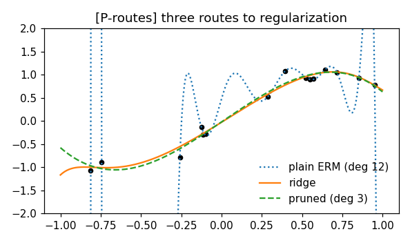
The three routes to regularization, each improving the error on unseen data points of the overfitting baseline: 1) model pruning — shrink the hypothesis space (here: fit a smaller-degree polynomial, i.e., constrain higher coefficients to zero); 2) loss penalization — add a penalty term (ridge); 3) data augmentation — enlarge the trainset with perturbed copies of its data points.
print("[P-routes] three routes, all improving the error on unseen "
      "data points")
# 1) model pruning: shrink the hypothesis space H to degree-3 polynomials
c3 = np.polyfit(xtr, ytr, 3)
va_prune = np.mean((yva - np.polyval(c3, xva)) ** 2)
# 2) loss penalization: ridge on the degree-12 model
lam = 1e-3
w_ridge = np.linalg.solve(V.T @ V / m + lam * np.eye(deg + 1),
                          V.T @ ytr / m)
va_ridge = np.mean((yva - Vva @ w_ridge) ** 2)
# 3) data augmentation: perturbed copies of the data points
reps = 100
sigma = 0.1
x_aug = np.concatenate([xtr + sigma * rng.normal(size=m)
                        for _ in range(reps)])
y_aug = np.tile(ytr, reps)
w_aug = np.linalg.lstsq(np.vander(x_aug, deg + 1), y_aug, rcond=None)[0]
va_aug = np.mean((yva - Vva @ w_aug) ** 2)
print(f"    error on unseen data points: ERM {va_erm:.2f} | "
      f"prune {va_prune:.3f} | ridge {va_ridge:.3f} | augment {va_aug:.3f}")
check("1) model pruning improves the error on unseen data points", va_prune < va_erm / 3)
check("2) loss penalization improves the error on unseen data points",
      va_ridge < va_erm / 3)
check("3) data augmentation improves the error on unseen data points",
      va_aug < va_erm / 3)
[P-routes] three routes, all improving the error on unseen data points
    error on unseen data points: ERM 11393397.53 | prune 0.042 | ridge 0.051 | augment 0.051
  [ok] 1) model pruning improves the error on unseen data points
  [ok] 2) loss penalization improves the error on unseen data points
  [ok] 3) data augmentation improves the error on unseen data points
The routes can coincide: data augmentation with zero-mean iid feature perturbations of variance sigma^2 yields (asymptotically in the number of perturbed copies) the same learned hypothesis as ridge regression with penalty sigma^2 ||w||^2 — verified by comparing the two learned parameter vectors.
print("[P-equiv] augmentation with sigma^2-noise = ridge with sigma^2")
# linear regression, feature perturbations with covariance sigma^2 I
mm, dd = 60, 3
X = rng.normal(size=(mm, dd))
y = X @ np.array([1.0, -0.5, 0.25]) + 0.1 * rng.normal(size=mm)
sig = 0.4
reps = 4000
Xa = np.vstack([X + sig * rng.normal(size=X.shape) for _ in range(reps)])
ya = np.tile(y, reps)
w_aug2 = np.linalg.lstsq(Xa, ya, rcond=None)[0]
w_ridge2 = np.linalg.solve(X.T @ X + sig**2 * mm * np.eye(dd),
                           X.T @ y)      # (X^T X + m sig^2 I)^{-1} X^T y
diff = np.linalg.norm(w_aug2 - w_ridge2)
print(f"    ||w_augment - w_ridge|| = {diff:.4f}")
check("the augmented-ERM solution matches the ridge solution",
      diff < 0.02)

# ------------------------------------------------------------ preview
fig, ax = plt.subplots(figsize=(5.4, 3.2))
xx = np.linspace(-1, 1, 300)
ax.plot(xtr, ytr, "ko", ms=4)
ax.plot(xx, np.polyval(w_erm, xx), ":", label="plain ERM (deg 12)")
ax.plot(xx, np.polyval(w_ridge, xx), "-", label="ridge")
ax.plot(xx, np.polyval(c3, xx), "--", label="pruned (deg 3)")
ax.set_ylim(-2, 2); ax.legend(frameon=False)
ax.set_xlabel("feature $x$"); ax.set_ylabel("label $y$")
ax.set_title("[P-routes] three routes to regularization")
fig.tight_layout()
fig.savefig(OUT_DIR / "regularization.png", dpi=110)
print(f"\n{sum(ok for _, ok in report)}/{len(report)} checks passed")
assert all(ok for _, ok in report)
[P-equiv] augmentation with sigma^2-noise = ridge with sigma^2
    ||w_augment - w_ridge|| = 0.0019
  [ok] the augmented-ERM solution matches the ridge solution

6/6 checks passed
P-equiv writes when the script runs