Dictionary of Applied Machine Learning
Updated on 2026-09-11
Typeset PDF version — the authoritative form of this entry
Python demo — a script that recomputes what this entry states and prints one line per check
The mean of a random vector $\featurevec$ is its expectation, the Lebesgue integral of $\featurevec$ with respect to its probability distribution. The term also refers to the sample mean, i.e., the average of the data points in a dataset. The two usages are consistent: the sample mean is the mean of the random vector obtained by drawing a data point uniformly from the dataset. Both usages share a further characterization: for a random vector with a finite second moment, the mean is the unique solution of a risk minimization problem under the squared error loss. For the random vector from a dataset, this optimization problem reduces to empirical risk minimization (ERM) in the simplest regression setting: predicting a numeric label without features, for which the learned hypothesis is the sample mean of the labels.
A weather station records the daily maximum temperature for a year. Adding the $365$ numbers and dividing by $365$ returns a single value that summarizes the whole record. This is the mean of the recorded numbers, and the same word names the corresponding quantity for a probability distribution.
P-defThe mean of a random vector $\featurevec$, which takes on values in a Euclidean space $\reals^{\featuredim}$, is its expectation $\expect\{\featurevec\}$. It is the Lebesgue integral of $\featurevec$ with respect to its probability distribution $\probdist$ (e.g., see (Billingsley, 1986) or (Rudin, 1987)), i.e., \[ \expect\{\featurevec\} = \int_{\reals^{\featuredim}} \featurevec \, \mathrm{d}\probdist(\featurevec) \text{.} \] Here, $\probdist$ is the probability distribution that $\featurevec$ induces on $\reals^{\featuredim}$, so the integral runs over the values $\featurevec$ takes rather than over the underlying sample space. No probability density function (pdf) need exist for the mean to be defined; when one does, denoted by $p$, it is $\int_{\reals^{\featuredim}} \featurevec \, p(\featurevec) \, \mathrm{d}\featurevec$.
P-argminThe term is also used to refer to the sample mean of a finite dataset
$\dataset = \left\{ \featurevec^{(1)}, \,\ldots, \,\featurevec^{(\samplesize)} \in \reals^{\featuredim}\right\}$.
These two usages are consistent. A dataset defines a
discrete random variable (discrete RV) $\widetilde{\featurevec}^{(\dataset)}=\featurevec^{(I)}$ on
the sample space $\{1, \,\ldots, \,\samplesize\}$. Here, the index $I$ is
chosen uniformly at random, i.e., $\prob{I=\sampleidx}=1/\samplesize$ for all
$\sampleidx=1,\ldots,\samplesize$. The mean of $\widetilde{\featurevec}^{(\dataset)}$ is
precisely the sample mean
\[
({1}/{\samplesize}) \sum_{\sampleidx=1}^{\samplesize}
\featurevec^{(\sampleidx)} \text{.}
\]
The probability distribution of $\widetilde{\featurevec}^{(\dataset)}$, which
places mass $1/\samplesize$ on each data point, is the
empirical distribution of the dataset.
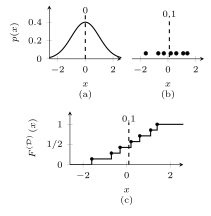
Fig. 1 shows both readings for a
real-valued random variable (RV) and a dataset of seven numbers, with the
empirical distribution drawn as its cumulative distribution function (cdf).
P-robustThis risk-minimization characterization applies directly to the
simplest machine learning (ML)
problem, predicting a numeric label without any
features. Consider a training set
$\trainset = \big\{ \truelabel^{(1)}, \,\ldots, \,\truelabel^{(\samplesize)} \big\}$
that consists of labels
$\truelabel^{(\sampleidx)} \in \reals$ only. A hypothesis
is then a single number $\hypothesis \in \reals$ that serves as
the prediction for every data point. Empirical risk minimization (ERM) with
the squared error loss searches over candidate hypotheses
$\hypothesis' \in \reals$ and learns
\[
\learnthypothesis
= \argmin_{\hypothesis' \in \reals}
\frac{1}{\samplesize} \sum_{\sampleidx=1}^{\samplesize}
\big(\truelabel^{(\sampleidx)} - \hypothesis'\big)^{2}
= \frac{1}{\samplesize} \sum_{\sampleidx=1}^{\samplesize}
\truelabel^{(\sampleidx)} \text{,}
\]
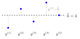
i.e., the learned hypothesis is the sample mean of
the labels (see Fig. 2). This setting
coincides with linear regression for data points that carry
the constant scalar feature $\feature = 1$.
pythondemos/mean.py).
Synonyms: expectation, expected value.
See also: random variable, random vector, expectation, sample mean, probability distribution, Lebesgue integral, empirical risk minimization, squared error loss, linear regression, median, trimmed mean.
@misc{dictml_mean,
  author = {Jung, Alexander},
  editor = {Olioumtsevits, Konstantina and Schnoor, Ekkehard},
  title = {mean},
  howpublished = {Dictionary of Applied Machine Learning (course edition)},
  year = {2026},
  doi = {10.5281/zenodo.21569296},
  note = {ISBN 978-952-64-3013-3, CC BY 4.0, retrieved 2026-09-21},
  url = {https://dictionaryofml.org/terms/mean.html}
}