Dictionary of Applied Machine Learning
Updated on 2026-09-21
Typeset PDF version — the authoritative form of this entry
Python demo — a script that recomputes what this entry states and prints one line per check
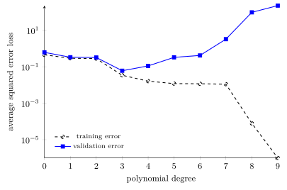
Overfitting is the failure mode of a machine learning (ML) method that fits its training set too closely: the learned hypothesis incurs a small empirical risk on the training set but a large risk, i.e., the expected loss on data points drawn from the underlying probability distribution. Consequently, the learned hypothesis has a large generalization gap. Validation detects overfitting by comparing the training error with the validation error obtained on a validation set. Overfitting typically arises when the hypothesis space is too large for the number of data points in the training set; the Vapnik–Chervonenkis dimension (VC dimension) and the Rademacher complexity measure that size. Regularization counteracts overfitting by pruning the model, adding a penalty term to the empirical risk, or augmenting the training set.
An image classifier that memorizes every photograph in its training set but fails to correctly classify unseen images is overfitting. In general, consider a machine learning (ML) method that uses empirical risk minimization (ERM) to learn a hypothesis $\learnthypothesis \in \hypospace$ with minimum empirical risk $\emprisk{\learnthypothesis}{\trainset}$ on a given training set $\trainset$. The method overfits $\trainset$ if the empirical risk $\emprisk{\learnthypothesis}{\trainset}$ is small while the risk $\risk{\learnthypothesis}$, i.e., the expected loss on data points drawn, independently of $\trainset$, from the underlying probability distribution, is large. Consequently, an overfitting ML method learns a hypothesis with a large generalization gap (Hastie et al., 2009, Sect. 7.2; Jung, 2022). A large generalization gap alone does not imply overfitting: a linear model, fitted to a small training set whose labels are noisy and depend nonlinearly on the features, can incur a large training error and a still larger risk, so the generalization gap is large while the training error is not small. The opposite failure is underfitting, where a hypothesis space holding no hypothesis that represents the relation between the features and the label of a data point leaves both quantities large.
Fig. 1 shows why a small training error is on its own no evidence against overfitting. Three data points lie on a straight line. None of the three curves is drawn by hand: each is a hypothesis $\learnthypothesis$ delivered by ERM with the squared error loss on those same three data points. What separates them is the hypothesis space that ERM searched, and the three are nested, $\hypospace^{(1)} \subset \hypospace^{(2)} \subset \hypospace^{(3)}$: $\hypospace^{(1)}$ is the constants $\hypothesis(\feature) = b$, $\hypospace^{(2)}$ the linear model, whose hypotheses are $\hypothesis(\feature) = \weight \feature + b$, and $\hypospace^{(3)}$ all continuous functions on $\reals$.
B-threeOn $\hypospace^{(1)}$, ERM has a unique solution: the constant
whose value is the average of the three labels. That constant
meets the middle data point and misses the other two, and no
member of $\hypospace^{(1)}$ does better. The hypothesis space is too
small here, and the method underfits. On $\hypospace^{(2)}$, the
solution is unique as well and attains a training error of zero;
the hypothesis space matches the relation between feature and
label, and the method neither underfits nor overfits. On
$\hypospace^{(3)}$, every continuous function through
the three data points attains a training error of zero, and
there are infinitely many of them: ERM has infinitely many
solutions there, and Fig. 1 draws
one of them. The training error cannot separate that curve from the
solution on $\hypospace^{(2)}$, the straight line on which the
three data points lie, and it cannot choose among the
solutions on $\hypospace^{(3)}$ either. The curve and the straight
line agree on the training set but differ at feature values
between those of the training data points, and the risk
registers this difference, since data points drawn from the
probability distribution also fall in that region. The hypothesis space is too
large here, and the method
overfits.
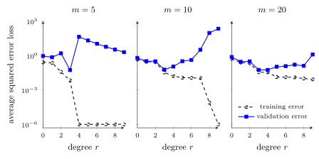
Fig. 2 illustrates overfitting for
polynomial regression. Each data point carries a single feature
$\feature$ and a noisy label $\truelabel$, drawn from a
probability distribution described in the caption. Polynomials of degree
$\polydegree = 0, \ldots, 9$ are fitted, using
ERM with the squared error loss, to training sets of
$\samplesize = 5$, $10$, and $20$ data points; each panel of
Fig. 2 shows the training error and the
validation error for one size. The training error decreases with
increasing degree in every panel: the polynomial of degree $9$ has
$10$ model parameters and interpolates the $\samplesize = 10$
data points; for $\samplesize = 5$, every degree from $4$ on
interpolates; for $\samplesize = 20$, no degree shown interpolates.
The validation error, obtained on a shared
validation set of $100$ data points, is in contrast smallest at
a moderate degree and grows by several orders of magnitude for
larger degrees: the high-degree polynomials overfit the
training set, and the gap between validation error and training error
estimates their large generalization gap. Comparing the three
training set sizes shows that the smaller the training set, the
lower the degree at which the validation error departs from the
training error: for $\samplesize = 5$, the validation error jumps by
nearly three orders of magnitude already at degree $4$, the lowest
degree whose $5$ model parameters suffice to interpolate the
training set; for $\samplesize = 20$, the validation error varies by
less than one order of magnitude across all degrees shown and, at
degree $9$, is smaller than the $\samplesize = 10$ validation error by
a factor of more than $100$.
pythondemos/overfitting.py
B-regRegularization counteracts overfitting in three elementary forms: pruning the model, adding a penalty term to the empirical risk, or augmenting the training set via data augmentation.
See also: empirical risk minimization, generalization gap, generalization, regularization, underfitting, validation, Vapnik–Chervonenkis dimension.
@misc{dictml_overfitting,
  author = {Jung, Alexander},
  editor = {Olioumtsevits, Konstantina and Schnoor, Ekkehard},
  title = {overfitting},
  howpublished = {Dictionary of Applied Machine Learning (course edition)},
  year = {2026},
  doi = {10.5281/zenodo.21569296},
  note = {ISBN 978-952-64-3013-3, CC BY 4.0, retrieved 2026-09-21},
  url = {https://dictionaryofml.org/terms/overfitting.html}
}