Dictionary of Applied Machine Learning · overfitting

overfitting — Python demo

Numerical companion to the entry overfitting: it recomputes what the entry states and prints one line per check

Run it with python3 overfitting.py, from any directory — it writes its output files into the current directory. Requires NumPy and Matplotlib only, and uses fixed seeds, so the printed numbers reproduce exactly. Download overfitting.py

The script, block by block

One cell per block of the script: the code, and what that code printed when it last ran here

setup

#!/usr/bin/env python3
"""
overfitting.py — Training error vs. validation error over polynomial degree.

This demo generates the data behind the figure in the "overfitting" entry
of the dictionary. It illustrates overfitting as a growing gap between a
small training error and a large validation error as the model capacity
(polynomial degree) increases.

Setup
-----
The true relationship between a scalar feature x and a label y is the
sinusoid  f(x) = sin(2*pi*x)  on x in [0, 1]. A training set of m = 10
data points is drawn uniformly on [0, 1] with additive Gaussian label
noise,  y = f(x) + eps,  eps ~ N(0, sigma^2),  sigma = 0.2. A validation
set of 100 data points is drawn from the same distribution.

For each polynomial degree r = 0, 1, ..., 9 a polynomial hypothesis is
learned by empirical risk minimization under the squared-error loss
(polynomial fit on the Vandermonde matrix). Degree r = 9 has 10 model
parameters and interpolates the m = 10 training points exactly.

Output
------
One CSV file (committed to the repo) is written to pythondemos/:
  overfitting_errors.csv  degree,trainerr,valerr
    trainerr — average squared-error loss on the training set
    valerr   — average squared-error loss on the validation set
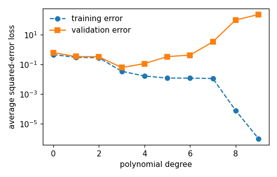
The training error decreases monotonically with the degree and reaches
(numerically) zero at r = 9, while the validation error passes through a
minimum at moderate degree and then grows by orders of magnitude: the
high-degree polynomials overfit the training set. The TikZ figure reads
the CSV via pgfplots (log-scaled y-axis), so the LaTeX build does not
depend on Python. A matplotlib preview is written to
pythondemos/overfitting.png.

Reproducibility
---------------
The numpy RNG is seeded from 5 (RNG = default_rng(5)) so re-running
produces bit-identical CSVs. Run from the repo root:

    python3 pythondemos/overfitting.py

Blocks
------
[B-data]    the sinusoid, the training set of m = 10 noisy data points, and
            the validation set of 100 data points from the same distribution
[B-sweep]   ERM with the squared-error loss over polynomials of degree
            0, ..., 9: training error falls monotonically to zero, validation
            error passes through a minimum and then grows
[B-output]  the committed CSV and the matplotlib preview
"""
from __future__ import annotations

from pathlib import Path

import numpy as np
import matplotlib

matplotlib.use("Agg")
import matplotlib.pyplot as plt

OUTDIR = Path(__file__).resolve().parent
RNG = np.random.default_rng(5)

M_TRAIN = 10
M_VAL = 100
SIGMA = 0.2
MAX_DEGREE = 9


def f_true(x: np.ndarray) -> np.ndarray:
    return np.sin(2.0 * np.pi * x)

B-data

the sinusoid, the training set of m = 10 noisy data points, and the validation set of 100 data points from the same distribution

x_train = RNG.uniform(0.0, 1.0, M_TRAIN)
y_train = f_true(x_train) + SIGMA * RNG.standard_normal(M_TRAIN)
x_val = RNG.uniform(0.0, 1.0, M_VAL)
y_val = f_true(x_val) + SIGMA * RNG.standard_normal(M_VAL)

B-sweep

ERM with the squared-error loss over polynomials of degree 0, ..., 9: training error falls monotonically to zero, validation error passes through a minimum and then grows

degrees = np.arange(MAX_DEGREE + 1)
trainerr = np.empty_like(degrees, dtype=float)
valerr = np.empty_like(degrees, dtype=float)
for r in degrees:
    # ERM with the squared-error loss over polynomials of degree r,
    # loss over polynomials of degree r.
    coeffs = np.polynomial.polynomial.polyfit(x_train, y_train, int(r))
    yhat_train = np.polynomial.polynomial.polyval(x_train, coeffs)
    yhat_val = np.polynomial.polynomial.polyval(x_val, coeffs)
    trainerr[r] = np.mean((y_train - yhat_train) ** 2)
    valerr[r] = np.mean((y_val - yhat_val) ** 2)

# Floor the (numerically zero) interpolation error at degree 9 so the
# log-scaled pgfplots axis stays finite and readable.
trainerr = np.maximum(trainerr, 1e-6)

print("[B-sweep] degree  trainerr      valerr")
for r in degrees:
    print(f"{r:>16}  {trainerr[r]:.3e}  {valerr[r]:.3e}")

[B-sweep] degree  trainerr      valerr
               0  4.497e-01  6.121e-01
               1  2.916e-01  3.312e-01
               2  2.784e-01  3.205e-01
               3  3.401e-02  6.034e-02
               4  1.622e-02  1.108e-01
               5  1.185e-02  3.268e-01
               6  1.162e-02  4.155e-01
               7  1.102e-02  3.243e+00
               8  7.864e-05  9.588e+01
               9  1.000e-06  2.244e+02

B-output

the committed CSV and the matplotlib preview """ from __future__ import annotations from pathlib import Path import numpy as np import matplotlib matplotlib.use("Agg") import matplotlib.pyplot as plt

with (OUTDIR / "overfitting_errors.csv").open("w") as fh:
    fh.write("degree,trainerr,valerr\n")
    for r in degrees:
        fh.write(f"{r},{trainerr[r]:.6e},{valerr[r]:.6e}\n")

fig, ax = plt.subplots(figsize=(5, 3.2))
ax.semilogy(degrees, trainerr, "o--", label="training error")
ax.semilogy(degrees, valerr, "s-", label="validation error")
ax.set_xlabel("polynomial degree")
ax.set_ylabel("average squared-error loss")
ax.legend(frameon=False)
fig.tight_layout()
fig.savefig(OUTDIR / "overfitting.png", dpi=110)
print("[B-output] wrote overfitting_errors.csv and overfitting.png")

[B-output] wrote overfitting_errors.csv and overfitting.png