Python demo — a script that recomputes what this entry states and prints one line per check
The covariance matrix of a random vector consists of
the covariances between its entries. In particular,
the diagonal entries are the variances of the individual
entries. Together with the mean vector, the
covariance matrix collects the second-order
statistics of a random vector. For a Gaussian
random vector, the mean vector and the
covariance matrix provide full information about the optimal
method for linear regression: the model parameters of the optimal
linear hypothesis map, along with the incurred
risk, are computed from the entries of the covariance matrix.
Definition
P-mvnThe covariance matrix of
a random vector $\featurevec \in \reals^{\featuredim}$ is defined as
the expectation (if it exists):
\[\covmtx{\featurevec} \defeq \expect \bigg \{ \big( \featurevec - \expect \big\{ \featurevec \big\} \big)
\big(\featurevec - \expect \big\{ \featurevec \big\} \big)^{\top} \bigg\} \text{.}\]
The entry in row $\featureidx$ and column $\featureidx'$ is the
covariance of the entries $\feature_{\featureidx}$ and
$\feature_{\featureidx'}$, with the diagonal entries being the
variances
of the individual entries. A covariance matrix is always
positive semi-definite (psd). It is invertible, and then positive definite (pd), exactly
when no entry of $\featurevec$ is, with probability one,
an affine function of the other entries. Invertibility is
assumed wherever the inverse $\big( \covmtx{\featurevec} \big)^{-1}$
appears below. The empirical counterpart computed
from a dataset is the sample covariance matrix.
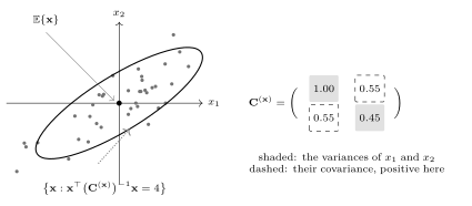
Fig. 1 shows how the entries of the
matrix are visible in a cloud of realizations: the
variances set the spread of the cloud along the two axes,
and the covariance sets its tilt.
Figure 1: Realizations of a random vector
$\featurevec \in \reals^{2}$, together with the ellipse
determined by their covariance matrix (shown on the
right). The ellipse is tilted because $\feature_{1}$ and
$\feature_{2}$ have a nonzero covariance; this
covariance appears as the off-diagonal entries of
the covariance matrix
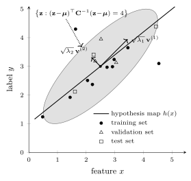
Fig. 2 illustrates the role of the
covariance matrix for a simple regression task. The
data points of a training set, a validation set and a
test set are modeled as realizations of i.i.d.
Gaussian random vectors
$\vz^{(\sampleidx)} = \big( \feature^{(\sampleidx)}, \truelabel^{(\sampleidx)} \big)^{\top} \sim \mvnormal{\meanvecgeneric}{\covmtxgeneric}$
(see multivariate normal distribution). The ellipse in
Fig. 2 is the constant-density contour
$\big\{ \vz : (\vz - \meanvecgeneric)^{\top} \covmtxgeneric^{-1} (\vz - \meanvecgeneric) = 4 \big\}$
of this probability distribution. Its principal axes point along the
eigenvectors $\vv^{(1)}, \vv^{(2)}$ of the covariance
matrix $\covmtxgeneric$, with lengths proportional to the
square roots
$\sqrt{\eigval{1}}, \sqrt{\eigval{2}}$ of the corresponding
eigenvalues (Bishop, 2006, Sect. 2.3) (see eigenvalue decomposition (EVD)).
The long axis of the ellipse
is the direction in which feature and label vary
together. The hypothesis map with the smallest
risk under the squared error loss is linear for this
probabilistic model, with slope given by the ratio of the
covariance between $\feature$ and $\truelabel$ to the
variance of $\feature$ (see linear regression).
Figure 2: Data points with a single feature $\feature$
and label $\truelabel$, modeled as realizations
of the Gaussian random vector
$\vz = (\feature, \truelabel)^{\top} \sim \mvnormal{\meanvecgeneric}{\covmtxgeneric}$,
split into a training set (filled circles), a validation set
(open triangles) and a test set (open squares). The
ellipse is a constant-density contour of the probability distribution;
its principal axes are the eigenvectors
$\vv^{(1)}, \vv^{(2)}$ of $\covmtxgeneric$, scaled by the
square roots of the eigenvalues
$\eigval{1}, \eigval{2}$. The hypothesis map
$\hypothesis(\feature)$ with the smallest risk under
the squared error loss is linear, with slope equal to the
covariance between $\feature$ and $\truelabel$ divided
by the variance of $\feature$
Predicting one feature of a data point from its other features
is a common task in health records
(Friedman et al., 2008): each data point is a
patient, the entries $\feature_{1}, \,\ldots, \,\feature_{\featuredim}$
of $\featurevec$ are biomarker measurements, and the biomarker
$\feature_{\featureidx}$ of a new patient, being expensive to
measure, is to be predicted from the remaining ones. The
smallest risk achievable by such a prediction is the
reciprocal of one diagonal entry of the
inverse $\big( \covmtx{\featurevec} \big)^{-1}$ of an
invertible covariance matrix, referred to as the precision
matrix (Bishop, 2006, Sect. 2.3.1). Collect the remaining features
in the vector
$\featurevec_{-\featureidx} \defeq \big( \feature_{1}, \,\ldots, \,\feature_{\featureidx-1}, \feature_{\featureidx+1}, \,\ldots, \,\feature_{\featuredim} \big)^{\top} \in \reals^{\featuredim-1}$.
For a Gaussian random vector
$\featurevec \sim \mvnormal{\meanvecgeneric}{\covmtx{\featurevec}}$
(see multivariate normal distribution), the conditional probability distribution of
$\feature_{\featureidx}$, given $\featurevec_{-\featureidx}$, is
Gaussian with a variance that does not depend on the value
of $\featurevec_{-\featureidx}$. This conditional variance
is
$1 \big/ \big( \big( \covmtx{\featurevec} \big)^{-1} \big)_{\featureidx,\featureidx}$
(Bishop, 2006, Sect. 2.3.1).
For data points modeled as realizations of i.i.d.
random vectors
$\featurevec^{(\sampleidx)} \sim \mvnormal{\meanvecgeneric}{\covmtx{\featurevec}}$,
this conditional variance is also the smallest risk
that any hypothesis can achieve under the squared error loss,
\[
\min_{\hypothesis: \reals^{\featuredim-1} \to \reals}
\expect \Big\{ \big( \feature_{\featureidx}
- \hypothesis\big(\featurevec_{-\featureidx}\big) \big)^{2} \Big\}
= 1 \big/ \big( \big( \covmtx{\featurevec} \big)^{-1}
\big)_{\featureidx,\featureidx} \text{,}
\]
i.e., the Bayes risk of this regression problem. It is
attained by the Bayes estimator
$\expect\{ \feature_{\featureidx} \mid \featurevec_{-\featureidx} \}$,
which depends linearly on $\featurevec_{-\featureidx}$
in the Gaussian case (Bertsekas and Tsitsiklis, 2008;
Bishop, 2006, Sect. 2.3.1). The diagonal of
$\big( \covmtx{\featurevec} \big)^{-1}$ therefore yields a
baseline, one entry per feature: a large diagonal
entry marks a biomarker that the remaining biomarkers predict
accurately, and no machine learning (ML) method can push the risk of
predicting that biomarker below the reciprocal of the entry.