pythondemos/evd.py).Dictionary of Applied Machine Learning
Updated on 2026-09-02
Typeset PDF version — the authoritative form of this entry
Python demo — a script that recomputes what this entry states and prints one line per check
An eigenvalue decomposition (EVD) is a factorization of a square matrix of the form $\mA = \mV \bm{\Lambda} \mV^{-1}$. The columns of the matrix $\mV$ are eigenvectors of $\mA$. The diagonal matrix $\bm{\Lambda}$ contains the eigenvalues corresponding to these eigenvectors. A matrix that admits an EVD is referred to as diagonalizable; symmetric matrices and matrices with distinct eigenvalues are diagonalizable. The EVD can speed up computations: given an EVD of the matrix $\featuremtx^{\top}\featuremtx$, each iteration of gradient descent (GD) for linear regression reduces to element-wise operations on vectors. The EVD of the Laplacian matrix of an undirected graph underlies spectral clustering: the second-smallest eigenvalue measures how well the graph is connected, and the signs of the entries of the corresponding eigenvector split the nodes into two clusters.
P-defAn EVD
for a square matrix $\mA \in \reals^{\featuredim \times \featuredim}$
is a factorization of the form
\[
\mA = \mV {\bm \Lambda} \mV^{-1} \text{.}
\]
The columns of the matrix $\mV = \big( \vv^{(1)}, \,\ldots, \,\vv^{(\featuredim)} \big)$ are the
eigenvectors of the matrix $\mA$. The diagonal matrix
${\bm \Lambda} = {\rm diag} \big\{ \eigval{1}, \,\ldots, \,\eigval{\featuredim} \big\}$
contains the eigenvalues $\eigval{\featureidx}$ corresponding to the eigenvectors $\vv^{(\featureidx)}$.
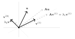
Multiplying the factorization by $\vv^{(\featureidx)}$ gives
$\mA \vv^{(\featureidx)} = \eigval{\featureidx} \vv^{(\featureidx)}$:
each eigenvector is a direction that $\mA$ only scales, by the
factor $\eigval{\featureidx}$. Fig. 1 shows the
two directions of the $2 \times 2$ matrix
\[
\mA = \begin{pmatrix} 1.3 & 0.8 \\ 0.4 & 0.9 \end{pmatrix}
\text{,}
\]
alongside a vector that $\mA$ does turn.
pythondemos/evd.py).
P-fastThe EVD can also speed up computations. Consider gradient descent (GD) for
linear regression, with the update
$\weights^{(\iteridx+1)} = \weights^{(\iteridx)} -
(2\lrate/\samplesize) \featuremtx^{\top}
\big( \featuremtx \weights^{(\iteridx)} - \labelvec \big)$
for the feature matrix $\featuremtx$ and label vector
$\labelvec$ of the training set (see linear regression). The
matrix $\featuremtx^{\top}\featuremtx$ is symmetric, so
it has an EVD
$\featuremtx^{\top}\featuremtx = \mV {\bm \Lambda} \mV^{\top}$
with an orthogonal matrix $\mV$. In the transformed
coordinates
$\widetilde{\weights}^{(\iteridx)} \defeq \mV^{\top} \weights^{(\iteridx)}$,
the update decouples into
\[
\widetilde{w}_{\featureidx}^{(\iteridx+1)} =
\big( 1 - (2\lrate/\samplesize) \eigval{\featureidx} \big)
\widetilde{w}_{\featureidx}^{(\iteridx)}
+ (2\lrate/\samplesize)
\big( \mV^{\top} \featuremtx^{\top} \labelvec \big)_{\featureidx}
\text{.}
\]
After the one-time computation of the EVD, each iteration
amounts to element-wise multiplication and addition of
vectors of length $\featuredim$
(pythondemos/evd.py).
P-specA concrete application of the EVD in machine learning (ML) is spectral clustering
(Luxburg, 2007). Consider data points represented as the
nodes $\nodeidx = 1, \,\ldots, \,\nrnodes$ of an
undirected graph $\graph$, e.g., the users of a social network
with edges given by friendships. The Laplacian matrix $\LapMat{\graph}$
of $\graph$ is symmetric and positive semi-definite (psd). Its EVD therefore uses an
orthogonal matrix of eigenvectors,
$\mV^{-1} = \mV^{\top}$, and real nonnegative eigenvalues,
ordered as
$0 = \eigval{1} \leq \eigval{2} \leq \ldots \leq \eigval{\nrnodes}$.
The second-smallest eigenvalue $\eigval{2}$ is the algebraic connectivity
of $\graph$: $\eigval{2} > 0$ if and only if $\graph$ is
connected, and $\eigval{2}$ close to zero indicates two subsets
of nodes joined by few edges (Fiedler, 1973). The corresponding
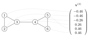
eigenvector $\vv^{(2)}$, referred to as the Fiedler vector,
assigns a number $v^{(2)}_{\nodeidx}$ to each node $\nodeidx$.
Grouping the nodes by the sign of $v^{(2)}_{\nodeidx}$ partitions the
nodes of $\graph$ into two clusters.
Fig. 2 shows this for a graph of six
nodes, two clusters of three nodes each joined by a
single edge: the entries of the Fiedler vector switch sign
exactly between the two clusters.
pythondemos/evd.py
@misc{dictml_evd,
  author = {Jung, Alexander},
  editor = {Olioumtsevits, Konstantina and Schnoor, Ekkehard},
  title = {eigenvalue decomposition},
  howpublished = {Dictionary of Applied Machine Learning (course edition)},
  year = {2026},
  doi = {10.5281/zenodo.21569296},
  note = {ISBN 978-952-64-3013-3, CC BY 4.0, retrieved 2026-09-22},
  url = {https://dictionaryofml.org/terms/evd.html}
}