P-prec writes when the script runsDictionary of Applied Machine Learning · covariance matrix
Numerical companion to the entry covariance matrix: it recomputes what the entry states and prints one line per check
One block per paragraph of the entry (marked [P...]): each block verifies numerically what the corresponding statement asserts. Self-contained (numpy/matplotlib only), fixed seed.
Run it without installing anything:uv run https://dictionaryofml.org/terms/covmtx.py
uv downloads this script and the pinned NumPy and Matplotlib it needs, then runs it; the script fetches any input file it uses. To keep the output files, download covmtx.py into a folder and run uv run covmtx.py there. With NumPy and Matplotlib already installed, python3 covmtx.py, from any directory — it writes its output files into the current directory. Fixed seeds, so the printed numbers reproduce exactly. Download covmtx.py · Notebook · Open in Colab
One cell per block of the script: the code, and what that code printed when it last ran here
"""
covmtx.py — numerical companion to the glossary entry 'covariance matrix'.

One block per paragraph of the entry (marked [P...]): each block verifies
numerically what the corresponding statement asserts. Self-contained
(numpy/matplotlib only), fixed seed.

Blocks
------
[P-def]  The covariance matrix C = E{(x - E x)(x - E x)^T}: the empirical
         outer-product average of iid draws from a random vector with
         analytic covariance A A^T recovers that matrix; its entry (j, j')
         is the covariance of entries j and j' (checked against np.cov),
         and its diagonal holds the per-entry variances.
[P-mvn]  The basic ML picture under a Gaussian model of (feature, label):
         the principal axes of the constant-density ellipse are the
         eigenvectors of the 2 x 2 covariance matrix — the draws'
         coordinates along them are uncorrelated with variances equal to
         the eigenvalues — and the smallest-risk hypothesis map is
         linear with slope cov(x, y)/var(x).
[P-prec] The diagonal of the inverse covariance matrix (the precision
         matrix): 1/(C^{-1})_{jj} equals the conditional variance of
         entry j given the remaining entries (the variance of the error
         of the best linear prediction of entry j from the rest), and on
         iid Gaussian draws the Bayes estimator E{x_j | rest} attains
         this value as its squared-error risk — the baseline that no
         prediction can beat; a constant prediction does worse.

Outputs
-------
covmtx.png : preview figure (checking only).

Data generated by pythondemos/covmtx.py.
"""

import numpy as np
import matplotlib

matplotlib.use("Agg")
import matplotlib.pyplot as plt
from pathlib import Path

OUT_DIR = Path(__file__).parent

rng = np.random.default_rng(42)
report = []


def check(name, ok):
    report.append((name, bool(ok)))
    print(f"  [{'ok' if ok else 'FAIL'}] {name}")
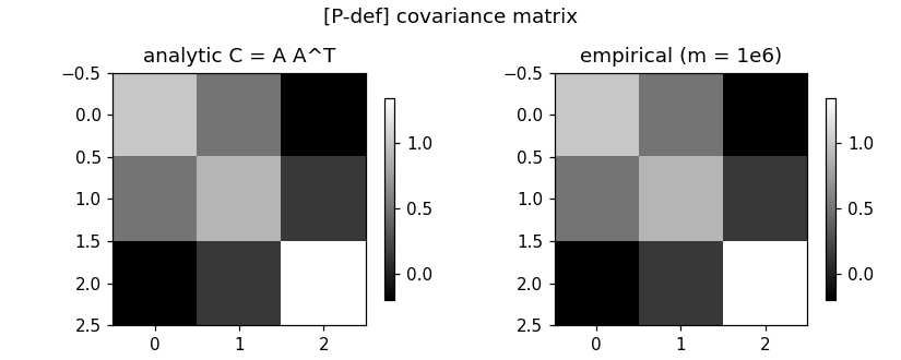
The covariance matrix C = E{(x - E x)(x - E x)^T}: the empirical outer-product average of iid draws from a random vector with analytic covariance A A^T recovers that matrix; its entry (j, j') is the covariance of entries j and j' (checked against np.cov), and its diagonal holds the per-entry variances.
print("[P-def] C = E{(x - Ex)(x - Ex)^T} — empirical vs analytic")
A = np.array([[1.0, 0.0, 0.0], [0.5, 0.8, 0.0], [-0.2, 0.3, 1.1]])
mu = np.array([2.0, -1.0, 0.5])
C = A @ A.T                                    # analytic covariance
m = 10**6
x = rng.standard_normal((m, 3)) @ A.T + mu
xc = x - x.mean(axis=0)                        # centered
C_emp = (xc[:, :, None] * xc[:, None, :]).mean(axis=0)
check("empirical outer-product average recovers C (|err| < 5e-3)",
      np.max(np.abs(C_emp - C)) < 5e-3)
check("matches np.cov (ddof=0)",
      np.allclose(C_emp, np.cov(x.T, ddof=0), atol=1e-9))
covs = np.array([[np.mean(xc[:, j] * xc[:, k]) for k in range(3)]
                 for j in range(3)])
check("entry (j, j') is the covariance of entries j and j'",
      np.allclose(covs, C_emp, atol=1e-12))
check("diagonal entries are the per-entry variances",
      np.allclose(np.diag(C_emp),
                  [np.mean(xc[:, j] ** 2) for j in range(3)], atol=1e-12))
[P-def] C = E{(x - Ex)(x - Ex)^T} — empirical vs analytic
  [ok] empirical outer-product average recovers C (|err| < 5e-3)
  [ok] matches np.cov (ddof=0)
  [ok] entry (j, j') is the covariance of entries j and j'
  [ok] diagonal entries are the per-entry variances
The basic ML picture under a Gaussian model of (feature, label): the principal axes of the constant-density ellipse are the eigenvectors of the 2 x 2 covariance matrix — the draws' coordinates along them are uncorrelated with variances equal to the eigenvalues — and the smallest-risk hypothesis map is linear with slope cov(x, y)/var(x).
print("[P-mvn] EVD of the covariance matrix gives the principal axes "
      "of the Gaussian density")
C2 = np.array([[1.0, 0.8], [0.8, 1.0]])        # (feature, label) covariance
mu2 = np.array([2.5, 3.0])
lam2, V2 = np.linalg.eigh(C2)
check("eigenvalues of the 2 x 2 covariance matrix are 0.2 and 1.8",
      np.allclose(lam2, [0.2, 1.8]))
z = rng.standard_normal((10**6, 2)) @ np.linalg.cholesky(C2).T + mu2
proj = (z - z.mean(axis=0)) @ V2               # coordinates on the axes
check("coordinates along the eigenvectors are uncorrelated",
      abs(np.mean(proj[:, 0] * proj[:, 1])) < 5e-3)
check("variance along each principal axis equals the eigenvalue",
      np.allclose(proj.var(axis=0), lam2, atol=5e-3))
slope_hat = np.polyfit(z[:, 0], z[:, 1], 1)[0]
check("smallest-risk linear slope matches cov(x, y)/var(x) = 0.8",
      abs(slope_hat - C2[0, 1] / C2[0, 0]) < 5e-3)
[P-mvn] EVD of the covariance matrix gives the principal axes of the Gaussian density
  [ok] eigenvalues of the 2 x 2 covariance matrix are 0.2 and 1.8
  [ok] coordinates along the eigenvectors are uncorrelated
  [ok] variance along each principal axis equals the eigenvalue
  [ok] smallest-risk linear slope matches cov(x, y)/var(x) = 0.8
The diagonal of the inverse covariance matrix (the precision matrix): 1/(C^{-1})_{jj} equals the conditional variance of entry j given the remaining entries (the variance of the error of the best linear prediction of entry j from the rest), and on iid Gaussian draws the Bayes estimator E{x_j | rest} attains this value as its squared-error risk — the baseline that no prediction can beat; a constant prediction does worse.
print("[P-prec] diagonal of C^{-1}: conditional variance and "
      "squared-error baseline")
P = np.linalg.inv(C)
mse_bayes = np.empty(3)
for j in range(3):
    rest = [k for k in range(3) if k != j]
    # conditional variance of entry j given the rest = variance of the
    # error of the best linear prediction of entry j from the rest
    w = np.linalg.solve(C[np.ix_(rest, rest)], C[rest, j])
    cond_var = C[j, j] - C[rest, j] @ w
    check(f"entry {j}: 1/(C^-1)_jj equals the conditional variance",
          np.isclose(1 / P[j, j], cond_var))
    # Bayes estimator E{x_j | rest} is linear in the Gaussian case; its
    # squared-error risk on iid Gaussian draws attains the baseline
    pred = mu[j] + (x[:, rest] - mu[rest]) @ w
    mse_bayes[j] = np.mean((x[:, j] - pred) ** 2)
    check(f"entry {j}: risk of the Bayes estimator matches 1/(C^-1)_jj",
          abs(mse_bayes[j] - 1 / P[j, j]) < 1e-2)
mse_const = np.mean((x[:, 0] - mu[0]) ** 2)    # constant prediction
check("constant prediction of entry 0 has larger risk than the baseline",
      mse_const > 1 / P[0, 0])

# ------------------------------------------------------------ preview
fig, ax = plt.subplots(1, 4, figsize=(13.6, 3.0))
for a, M, t in ((ax[0], C, "analytic C = A A^T"),
                (ax[1], C_emp, "empirical (m = 1e6)")):
    im = a.imshow(M, cmap="gray")
    a.set_title(t)
    fig.colorbar(im, ax=a, shrink=0.8)
zs = z[:400]
ax[2].plot(zs[:, 0], zs[:, 1], ".", color="0.6", ms=2)
ang = np.linspace(0, 2 * np.pi, 100)
ell = mu2[:, None] + V2 @ (np.sqrt(lam2)[:, None]
                           * np.vstack([np.cos(ang), np.sin(ang)]))
ax[2].plot(ell[0], ell[1], "k-", lw=1.5)
for lam_i, v_i in zip(lam2, V2.T):
    ax[2].annotate("", xy=mu2 + np.sqrt(lam_i) * v_i, xytext=mu2,
                   arrowprops=dict(arrowstyle="->", lw=1.5))
xg = np.linspace(z[:, 0].min(), z[:, 0].max(), 2)
ax[2].plot(xg, C2[0, 1] / C2[0, 0] * (xg - mu2[0]) + mu2[1], "--",
           color="C1", label="hypothesis map")
ax[2].set_xlabel("feature x")
ax[2].set_ylabel("label y")
ax[2].set_title("[P-mvn] principal axes from the EVD")
ax[2].legend(frameon=False)
jj = np.arange(3)
ax[3].bar(jj - 0.18, np.diag(C), width=0.36, color="C0", hatch="//",
          label="variance $C_{j,j}$")
ax[3].bar(jj + 0.18, 1 / np.diag(P), width=0.36, color="C1",
          label="baseline $1/(C^{-1})_{j,j}$")
ax[3].set_xlabel("entry j")
ax[3].set_ylabel("squared-error risk")
ax[3].set_title("[P-prec] baseline from $C^{-1}$")
ax[3].legend(frameon=False)
fig.suptitle("covariance matrix, Gaussian principal axes, and the "
             "$C^{-1}$ baseline")
fig.tight_layout()
fig.savefig(OUT_DIR / "covmtx.png", dpi=110)
print(f"\n{sum(ok for _, ok in report)}/{len(report)} checks passed")
assert all(ok for _, ok in report)
[P-prec] diagonal of C^{-1}: conditional variance and squared-error baseline
  [ok] entry 0: 1/(C^-1)_jj equals the conditional variance
  [ok] entry 0: risk of the Bayes estimator matches 1/(C^-1)_jj
  [ok] entry 1: 1/(C^-1)_jj equals the conditional variance
  [ok] entry 1: risk of the Bayes estimator matches 1/(C^-1)_jj
  [ok] entry 2: 1/(C^-1)_jj equals the conditional variance
  [ok] entry 2: risk of the Bayes estimator matches 1/(C^-1)_jj
  [ok] constant prediction of entry 0 has larger risk than the baseline

15/15 checks passed
P-prec writes when the script runs