P15 writes when the script runsDictionary of Applied Machine Learning · linear regression
Numerical companion to the entry linear regression: it recomputes what the entry states and prints one line per check
One block per paragraph of the entry (marked [P1], [P2], ...): each block verifies numerically what the corresponding paragraph claims, so the entry's statements are backed by a small reproducible experiment. Self-contained (numpy/matplotlib only), fixed seed.
Run it without installing anything:uv run https://dictionaryofml.org/terms/linreg.py
uv downloads this script and the pinned NumPy and Matplotlib it needs, then runs it; the script fetches any input file it uses. To keep the output files, download linreg.py into a folder and run uv run linreg.py there. With NumPy and Matplotlib already installed, python3 linreg.py, from any directory — it writes its output files into the current directory. Fixed seeds, so the printed numbers reproduce exactly. Download linreg.py · Notebook · Open in Colab
One cell per block of the script: the code, and what that code printed when it last ran here
"""
linreg.py — numerical companion to the glossary entry 'linear regression'.

Purpose
-------
One block per paragraph of the entry (marked [P1], [P2], ...): each block
verifies numerically what the corresponding paragraph claims, so the entry's
statements are backed by a small reproducible experiment. Self-contained
(numpy/matplotlib only), fixed seed.

Blocks
------
[P1/P2]  Prediction of a numeric label via h(x) = w^T x; constant feature
         as intercept.
[P3]     Least-squares ERM; the entry's Fig. panel (a): with the constant
         feature x = 1 and labels (2, 3, 4), the solution is the average 3.
[P4-P6]  Matrix form f(w) = (1/m)||y - Xw||^2; normal equations
         X^T X w = X^T y; unique closed-form solution under full column rank.
[P7]     Underdetermined case m < d: two solutions with identical training
         loss but different predictions (the generalization issue); ridge
         (l2 penalty, closed form) and Lasso (l1 penalty, proximal GD /
         ISTA) as regularized variants.
[P8]     Statistical interpretation: for jointly Gaussian (x, y) the Bayes
         estimator has w_star = C_x^{-1} c_xy; least squares recovers it
         from a large sample.
[P9-P12] GD step operator F^(eta)(w) = w - eta grad f(w): fixed points solve
         the normal equations; contraction w.r.t. the Euclidean norm for
         0 < eta < m / lambda_max; convergence speed governed by the
         condition number lambda_max / lambda_min  ->  linreg_gdconv.csv.
[P13]    Online GD / LMS: one GD step per arriving data point.
[P14]    Stability: label-only perturbation, Delta w = X^+ Delta y, the
         spectral-norm bound, and the entry's Fig. panel (b) numbers
         (Delta y^(3) = 6 shifts the average from 3 to 5).
[P15]    Perturbed online GD update = clean update + perturbation term.

Outputs
-------
linreg_gdconv.csv : GD suboptimality per iteration for a well-conditioned
                    and an ill-conditioned feature matrix (columns:
                    iter, wellcond, illcond).
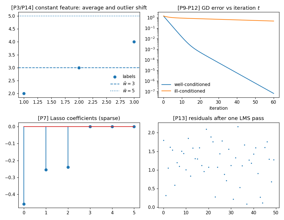
linreg.png        : 2x2 preview figure (checking only).
"""

import numpy as np
import matplotlib

matplotlib.use("Agg")
import matplotlib.pyplot as plt

from pathlib import Path

OUT_DIR = Path(__file__).parent

rng = np.random.default_rng(42)
report = []


def check(name, ok):
    report.append((name, bool(ok)))
    print(f"  [{'ok' if ok else 'FAIL'}] {name}")


# ===========================================================================
Linear regression predicts a numeric label from features via the
# linear hypothesis map h(x) = w^T x. A constant feature makes it affine.
# ===========================================================================
print("[P1/P2] linear hypothesis map with intercept via constant feature")
m, d = 50, 3
w_true = np.array([0.8, -0.5, 2.0, 10.0])          # last entry: intercept
X_raw = rng.normal(size=(m, d))                     # "weather measurements"
X = np.hstack([X_raw, np.ones((m, 1))])             # append constant feature
y = X @ w_true + 0.1 * rng.normal(size=m)           # tomorrow's temperature
x_new = np.append(rng.normal(size=d), 1.0)
check("h(x) = w^T x yields a numeric label", np.isscalar((w_true @ x_new).item()))

# ===========================================================================
[P1/P2] linear hypothesis map with intercept via constant feature
  [ok] h(x) = w^T x yields a numeric label
Least squares as ERM; entry Fig. panel (a): with the constant scalar
# feature x = 1 and labels (2, 3, 4), the minimizer is the average 3.
# ===========================================================================
print("[P3] constant-feature special case reduces to the average")
y_fig = np.array([2.0, 3.0, 4.0])
X_fig = np.ones((3, 1))
w_avg = np.linalg.lstsq(X_fig, y_fig, rcond=None)[0].item()
check("average = 3 as in Fig. panel (a)", np.isclose(w_avg, 3.0))

# ===========================================================================
[P3] constant-feature special case reduces to the average
  [ok] average = 3 as in Fig. panel (a)
Matrix form, normal equations, unique closed-form solution when
# X has full column rank (m >= d).
# ===========================================================================
print("[P4-P6] normal equations and closed-form solution")
G = X.T @ X                                          # X^T X
w_hat = np.linalg.solve(G, X.T @ y)                  # closed form
check("normal equations X^T X w = X^T y hold", np.allclose(G @ w_hat, X.T @ y))
check("closed form matches lstsq", np.allclose(w_hat, np.linalg.lstsq(X, y, rcond=None)[0]))
check("full column rank (m >= d)", np.linalg.matrix_rank(X) == X.shape[1])


def f_avg(Xm, ym, w):
    return np.mean((ym - Xm @ w) ** 2)


# ===========================================================================
[P4-P6] normal equations and closed-form solution
  [ok] normal equations X^T X w = X^T y hold
  [ok] closed form matches lstsq
  [ok] full column rank (m >= d)
Underdetermined m < d: many solutions tie on the training set but
# predict differently outside it; ridge and Lasso as regularized variants.
# ===========================================================================
print("[P7] underdetermined case, ridge, Lasso")
m_u, d_u = 3, 6
X_u = rng.normal(size=(m_u, d_u))
y_u = rng.normal(size=m_u)
w_min = np.linalg.pinv(X_u) @ y_u                    # minimum-norm solution
null_dir = np.linalg.svd(X_u)[2][-1]                 # a null-space direction
w_alt = w_min + 5.0 * null_dir                       # second solution
check("both solutions fit the trainset exactly",
      np.allclose(X_u @ w_min, y_u) and np.allclose(X_u @ w_alt, y_u))
x_out = rng.normal(size=d_u)
check("but they predict differently outside it",
      abs(x_out @ w_min - x_out @ w_alt) > 1e-3)

alpha = 0.1
w_ridge = np.linalg.solve(X_u.T @ X_u + alpha * m_u * np.eye(d_u), X_u.T @ y_u)
check("ridge (l2 penalty) solution is unique/well-defined",
      np.all(np.isfinite(w_ridge)))


def ista(Xm, ym, alpha, iters=2000):
    """Proximal GD (ISTA) for the Lasso: average sqerrloss + alpha*||w||_1."""
    mm = Xm.shape[0]
    L = 2.0 * np.linalg.eigvalsh(Xm.T @ Xm).max() / mm
    w = np.zeros(Xm.shape[1])
    for _ in range(iters):
        g = w - (2.0 / (mm * L)) * Xm.T @ (Xm @ w - ym)
        w = np.sign(g) * np.maximum(np.abs(g) - alpha / L, 0.0)
    return w


w_lasso = ista(X_u, y_u, alpha)
check("Lasso (l1 penalty) drives entries to exactly zero",
      np.sum(np.isclose(w_lasso, 0.0)) > 0)

# ===========================================================================
[P7] underdetermined case, ridge, Lasso
  [ok] both solutions fit the trainset exactly
  [ok] but they predict differently outside it
  [ok] ridge (l2 penalty) solution is unique/well-defined
  [ok] Lasso (l1 penalty) drives entries to exactly zero
Statistical interpretation: jointly Gaussian (x, y) with zero mean;
# Bayes estimator w_star = C_x^{-1} c_xy; least squares recovers it from a
# large sample.
# ===========================================================================
print("[P8] Bayes estimator from covariances vs sample-based least squares")
d_g = 3
A = rng.normal(size=(d_g, d_g))
C_x = A @ A.T + d_g * np.eye(d_g)                    # invertible covariance
w_pop = np.array([1.0, -2.0, 0.5])
m_big = 200_000
X_g = rng.multivariate_normal(np.zeros(d_g), C_x, size=m_big)
y_g = X_g @ w_pop + rng.normal(size=m_big)           # zero-mean jointly Gaussian
c_xy = C_x @ w_pop                                   # E[x y]
w_star = np.linalg.solve(C_x, c_xy)
w_ls = np.linalg.solve(X_g.T @ X_g, X_g.T @ y_g)
check("w_star = C_x^{-1} c_xy equals the population weights",
      np.allclose(w_star, w_pop))
check("sample least squares approximates w_star (m = 2e5)",
      np.allclose(w_ls, w_star, atol=2e-2))

# ===========================================================================
[P8] Bayes estimator from covariances vs sample-based least squares
  [ok] w_star = C_x^{-1} c_xy equals the population weights
  [ok] sample least squares approximates w_star (m = 2e5)
GD step operator: fixed points = normal-equation solutions;
# contraction w.r.t. the Euclidean norm for 0 < eta < m/lambda_max; speed
# governed by the condition number  ->  linreg_gdconv.csv.
# ===========================================================================
print("[P9-P12] GD step operator, contraction, condition number")
lam = np.linalg.eigvalsh(G)
lam_max, lam_min = lam.max(), lam.min()
eta = 0.9 * m / lam_max                              # 0 < eta < m/lambda_max


def gdstep(Xm, ym, eta_, w):
    mm = Xm.shape[0]
    return w + (2.0 * eta_ / mm) * Xm.T @ (ym - Xm @ w)


check("w_hat is a fixed point of the GD step operator",
      np.allclose(gdstep(X, y, eta, w_hat), w_hat))
wa, wb = rng.normal(size=d + 1), rng.normal(size=d + 1)
q = np.max(np.abs(1.0 - 2.0 * eta * lam / m))        # contraction factor
check("contraction w.r.t. the Euclidean norm with factor < 1",
      (np.linalg.norm(gdstep(X, y, eta, wa) - gdstep(X, y, eta, wb))
       <= q * np.linalg.norm(wa - wb) + 1e-12) and q < 1)


def gd_curve(Xm, ym, iters=60):
    Gm = Xm.T @ Xm
    lmax = np.linalg.eigvalsh(Gm).max()
    eta_ = 0.9 * Xm.shape[0] / lmax
    wh = np.linalg.solve(Gm, Xm.T @ ym)
    w = np.zeros(Xm.shape[1])
    errs = []
    for _ in range(iters + 1):
        errs.append(np.linalg.norm(w - wh))
        w = gdstep(Xm, ym, eta_, w)
    return np.array(errs)


X_well = rng.normal(size=(200, 2))                   # cond(X^T X) close to 1
scales = np.array([1.0, 12.0])
X_ill = X_well * scales                              # cond larger by ~144
err_well = gd_curve(X_well, X_well @ np.ones(2))
err_ill = gd_curve(X_ill, X_ill @ np.ones(2))
check("larger condition number slows GD convergence",
      err_ill[-1] > err_well[-1])
iters = np.arange(len(err_well))
np.savetxt(OUT_DIR / "linreg_gdconv.csv",
           np.column_stack([iters, err_well, err_ill]),
           delimiter=",", header="iter,wellcond,illcond", comments="")

# ===========================================================================
[P9-P12] GD step operator, contraction, condition number
  [ok] w_hat is a fixed point of the GD step operator
  [ok] contraction w.r.t. the Euclidean norm with factor < 1
  [ok] larger condition number slows GD convergence
Online GD / LMS: one GD step per arriving data point.
# ===========================================================================
print("[P13] online GD (LMS) on streaming data points")
w_on = np.zeros(d + 1)
eta_on = 0.02
for t in range(m):
    x_t, y_t = X[t], y[t]
    w_on = w_on + 2.0 * eta_on * (y_t - w_on @ x_t) * x_t
err_online_final = np.linalg.norm(w_on - w_hat)
check("one pass of LMS approaches the least-squares solution",
      err_online_final < 0.5 * np.linalg.norm(w_hat))

# ===========================================================================
[P13] online GD (LMS) on streaming data points
  [ok] one pass of LMS approaches the least-squares solution
Stability under a label-only perturbation: Delta w = X^+ Delta y,
# the spectral-norm bound, and the entry's Fig. panel (b) numbers.
# ===========================================================================
print("[P14] label perturbation: pseudoinverse formula and bound")
dy = rng.normal(size=m)
w_pert = np.linalg.solve(G, X.T @ (y + dy))
X_pinv = np.linalg.pinv(X)
check("Delta w = X^+ Delta y", np.allclose(w_pert - w_hat, X_pinv @ dy))
check("||Delta w|| <= ||X^+||_2 ||Delta y||",
      np.linalg.norm(w_pert - w_hat)
      <= np.linalg.norm(X_pinv, 2) * np.linalg.norm(dy) + 1e-12)
dy_fig = np.array([0.0, 0.0, 6.0])                   # Fig. panel (b)
shift = (np.linalg.pinv(X_fig) @ dy_fig).item()
check("Fig. panel (b): Delta y^(3) = 6 shifts the average by 2 (3 -> 5)",
      np.isclose(shift, 2.0) and np.isclose(w_avg + shift, 5.0))

# ===========================================================================
[P14] label perturbation: pseudoinverse formula and bound
  [ok] Delta w = X^+ Delta y
  [ok] ||Delta w|| <= ||X^+||_2 ||Delta y||
  [ok] Fig. panel (b): Delta y^(3) = 6 shifts the average by 2 (3 -> 5)
Perturbed online GD update = clean update + perturbation term.
# ===========================================================================
print("[P15] perturbed online GD update decomposition")
t = 7
dx_t, dy_t = 0.05 * rng.normal(size=d + 1), 0.3
x_t, y_t = X[t], y[t]
w_cur = rng.normal(size=d + 1)
upd_pert = w_cur + 2 * eta_on * ((y_t + dy_t) - w_cur @ (x_t + dx_t)) * (x_t + dx_t)
upd_clean = w_cur + 2 * eta_on * (y_t - w_cur @ x_t) * x_t
eps = upd_pert - upd_clean                           # perturbation term
check("perturbed update = clean update + perturbation term (depends on "
      "the data-point perturbation and the current w)",
      np.allclose(upd_pert, upd_clean + eps))

# ===========================================================================
# Preview figure (checking only)
# ===========================================================================
fig, ax = plt.subplots(2, 2, figsize=(9, 7))
ax[0, 0].scatter([1, 2, 3], y_fig, label="labels")
ax[0, 0].axhline(w_avg, ls="--", label=r"$\hat w = 3$")
ax[0, 0].axhline(w_avg + shift, ls=":", label=r"$\tilde w = 5$")
ax[0, 0].set_title("[P3/P14] constant feature: average and outlier shift")
ax[0, 0].set_xlabel("data point index $r$")
ax[0, 0].set_ylabel("label $y$")
ax[0, 0].legend(frameon=False)
ax[0, 1].semilogy(iters, err_well, label="well-conditioned")
ax[0, 1].semilogy(iters, err_ill, "--", label="ill-conditioned")
ax[0, 1].set_title(r"[P9-P12] GD error vs iteration $t$")
ax[0, 1].set_xlabel("iteration")
ax[0, 1].set_ylabel("error")
ax[0, 1].legend(frameon=False)
ax[1, 0].stem(w_lasso)
ax[1, 0].set_title("[P7] Lasso coefficients (sparse)")
ax[1, 0].set_xlabel("coefficient index $j$")
ax[1, 0].set_ylabel("coefficient value")
ax[1, 1].plot(np.abs(X @ w_on - y), ".", ms=3)
ax[1, 1].set_title("[P13] residuals after one LMS pass")
ax[1, 1].set_xlabel("data point index $r$")
ax[1, 1].set_ylabel("absolute residual")
fig.tight_layout()
fig.savefig(OUT_DIR / "linreg.png", dpi=110)

n_fail = sum(1 for _, ok in report if not ok)
print(f"\n{len(report)} checks, {n_fail} failed.")
raise SystemExit(1 if n_fail else 0)
[P15] perturbed online GD update decomposition
  [ok] perturbed update = clean update + perturbation term (depends on the data-point perturbation and the current w)

19 checks, 0 failed.
P15 writes when the script runs