Dictionary of Applied Machine Learning
Updated on 2026-09-18
Typeset PDF version — the authoritative form of this entry
Python demo — a script that recomputes what this entry states and prints one line per check
A subset of the Euclidean space is convex if it contains the line segment between any two of its points. A function is convex if its epigraph is a convex set. A convex optimization problem is the minimization of a convex function over a convex set. Empirical risk minimization (ERM) is a convex optimization problem whenever the hypothesis space is parameterized by a convex set of model parameters and the loss function is convex in those model parameters. Any local minimizer of a convex objective function is necessarily also a global minimizer, so a method that reaches a local minimum has solved the optimization problem.
Many machine learning (ML) methods learn model parameters by an iterative optimization method: each iteration updates the current model parameters to reduce an objective function within a neighborhood of these model parameters. Widely used examples are gradient descent (GD) and its variants.
B-fnThese optimization methods work particularly well when the objective function is a convex function of the model parameters. Indeed, for a convex function every local minimum is necessarily a global minimum: any choice of model parameters at which no small change reduces the objective function already attains the smallest value that the objective function takes anywhere. The average squared error loss of linear regression is a convex function of the model parameters, and so is the objective function of the support vector machine (SVM). For differentiable convex objective functions and suitable step size choices, GD converges to such a minimum (Boyd and Vandenberghe, 2004).
B-epiConvexity is defined both for sets and for functions.
For sets, the definition is geometric.
A subset $\mathcal{C} \subseteq \reals^{\featuredim}$ of the
Euclidean space $\reals^{\featuredim}$ is referred to
as convex if it contains the line segment between any two points
$\weights, \weights' \in \mathcal{C}$ in that set, i.e.,
\[ \expcoeff \weights + (1-\expcoeff) \weights' \in \mathcal{C}
\quad \text{for all } \expcoeff \in [0,1] \text{.} \]
Similarly, a function
$f: \reals^{\featuredim} \rightarrow \reals$
is convex if its epigraph
$\big\{ \big( \weights^{\top},t \big)^{\top} \in \reals^{\featuredim+1} : t \geq f(\weights) \big\}$
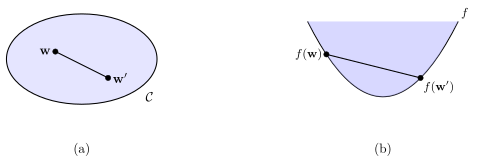
is a convex set (Boyd and Vandenberghe, 2004). Examples of a convex set
and of a convex function are illustrated in
Fig. 1.
Halfspaces are not merely one example among others: every
closed convex set is given by the intersection of all halfspaces
that contain it (Boyd and Vandenberghe, 2004, Sect. 2.3.1;
Rockafellar, 1970, Thm. 11.5)
\begin{equation}
\label{equ_halfspace_intersection_dict}
\mathcal{C} = \bigcap \big\{ \mathcal{H} \subseteq \reals^{\featuredim}
\;:\; \mathcal{H} \text{ is a halfspace}, \; \mathcal{C} \subseteq \mathcal{H} \big\}
\text{.}
\end{equation}
In general, intersecting
a subset of the halfspaces containing a convex set yields a
convex set that contains the original one, i.e., an outer
approximation (see Fig. 2).
B-halfReturning to the halfspace intersection \(\eqref{equ_halfspace_intersection_dict}\), that intersection can be narrowed: it needs to consider only those halfspaces that are bounded by a supporting hyperplane. Every boundary
point of a non-empty convex set carries such a hyperplane
(Boyd and Vandenberghe, 2004, Sect. 2.5.2), and each point outside the
set is already excluded by one of the halfspaces that these
supporting hyperplanes bound:
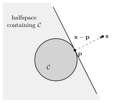
for a point $\vx \notin \mathcal{C}$ and $\mathcal{C}$ closed, there is
a unique nearest point $\vp \in \mathcal{C}$ to $\vx$. That nearest
point is a boundary point of $\mathcal{C}$, and therefore one of
the points that carry a supporting hyperplane: a point of the
interior could be moved a little toward $\vx$ and would still lie in
$\mathcal{C}$, so it would not be the nearest one. The
hyperplane through $\vp$
with normal vector $\vx - \vp$ supports $\mathcal{C}$ at $\vp$,
and the halfspace it bounds contains $\mathcal{C}$ but not
$\vx$ (see Fig. 3).
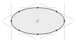
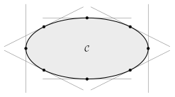
Fig. 4 shows eight supporting hyperplanes
of an ellipse.
Of the two families of convex sets introduced above, the convex hull is the one that characterizes the linear separability of data points with binary label values. Consider $\samplesize$ data points with feature vectors $\featurevec^{(\sampleidx)} \in \reals^{\featuredim}$ and labels $\truelabel^{(\sampleidx)} \in \{-1,+1\}$, for $\sampleidx = 1, \ldots, \samplesize$. These data points are linearly separable if some linear classifier predicts every label correctly, i.e., there are $\weights \in \reals^{\featuredim} \setminus \{\mathbf{0}\}$ and $\offset \in \reals$ with $\truelabel^{(\sampleidx)} \big( \weights^{\top} \featurevec^{(\sampleidx)} + \offset \big) > 0$ for $\sampleidx = 1, \ldots, \samplesize$. This holds precisely when the convex hull of the feature vectors labeled $+1$ and the convex hull of those labeled $-1$ do not intersect (Boyd and Vandenberghe, 2004, Sect. 8.6.1). Separability is therefore a property of two convex sets built from the data points.
Convexity also appears in the study of probabilistic models, where it singles out a widely used family. In particular, an exponential family is constituted by the probability distributions whose probability density function (pdf) has the form \[ p(\featurevec; \weights) = h(\featurevec) \exp\big(\weights^{\top} \suffstat(\featurevec) - A(\weights)\big) \text{.} \] This pdf is parameterized by the vector $\weights$ and the sufficient statistics $\suffstat(\cdot)$. The log-partition function $A$ is fully determined by requiring $p(\featurevec; \weights)$ to integrate to one. Its Hessian is the covariance matrix of the sufficient statistics $\suffstat(\featurevec)$ under $p(\featurevec; \weights)$, \[ \nabla^{2} A(\weights) = \E \big\{ \suffstat(\featurevec) \suffstat(\featurevec)^{\top} \big\} - \E \big\{ \suffstat(\featurevec) \big\} \E \big\{ \suffstat(\featurevec) \big\}^{\top} \text{,} \] which is positive semi-definite (psd). A twice-differentiable function whose Hessian is psd is convex, so $A$ is a convex function on its domain (Wainwright and Jordan, 2008, Prop. 3.1). The convexity of $A$ implies that the negative log-likelihood function of a training set, up to an additive constant that does not depend on $\weights$, \[ - \sum_{\sampleidx=1}^{\samplesize} \weights^{\top} \suffstat\big(\featurevec^{(\sampleidx)}\big) + \samplesize A(\weights) \text{,} \] is a convex function of $\weights$. Thus, for an exponential family, maximum likelihood estimation is a convex optimization problem.
See also: Euclidean space, function, epigraph, convex optimization, minimum, objective function, halfspace, supporting hyperplane, Hessian.
@misc{dictml_convex,
  author = {Jung, Alexander},
  editor = {Olioumtsevits, Konstantina and Schnoor, Ekkehard},
  title = {convex},
  howpublished = {Dictionary of Applied Machine Learning (course edition)},
  year = {2026},
  doi = {10.5281/zenodo.21569296},
  note = {ISBN 978-952-64-3013-3, CC BY 4.0, retrieved 2026-09-21},
  url = {https://dictionaryofml.org/terms/convex.html}
}