P-euler writes when the script runsDictionary of Applied Machine Learning · gradient descent (GD)
Numerical companion to the entry gradient descent (GD): it recomputes what the entry states and prints one line per check
One block per claim of the entry (marked [P...]): each block verifies numerically what the corresponding statement asserts, so the entry's claims are backed by a small reproducible experiment. Self-contained (numpy/matplotlib only), fixed seed.
Run it without installing anything:uv run https://dictionaryofml.org/terms/gd.py
uv downloads this script and the pinned NumPy and Matplotlib it needs, then runs it; the script fetches any input file it uses. To keep the output files, download gd.py into a folder and run uv run gd.py there. With NumPy and Matplotlib already installed, python3 gd.py, from any directory — it writes its output files into the current directory. Fixed seeds, so the printed numbers reproduce exactly. Download gd.py · Notebook · Open in Colab
One cell per block of the script: the code, and what that code printed when it last ran here
"""
gd.py — numerical companion to the glossary entry 'gradient descent (GD)'.

Purpose
-------
One block per claim of the entry (marked [P...]): each block verifies
numerically what the corresponding statement asserts, so the entry's
claims are backed by a small reproducible experiment. Self-contained
(numpy/matplotlib only), fixed seed.

Blocks
------
[P-descent]  On a strongly convex quadratic f(w) = (1/m)||Xw - y||^2
             (the ERM objective of least-squares linear regression), the
             GD step w <- w - eta grad f(w) with eta = 1/L does not
             increase f at any iteration and converges to the unique
             minimizer w_hat = argmin f.
[P-rate]     For the convex L-smooth objective, the constant step eta=1/L
             obeys the suboptimality bound
                 f(w^(T)) - f* <= L ||w^(0) - w_hat||^2 / (2 T),
             i.e. the suboptimality falls in proportion to 1/T.
[P-momentum] Polyak's heavy-ball momentum
                 w^(t+1) = w^(t) - eta grad f(w^(t)) + beta (w^(t) - w^(t-1)),
             which combines gradients over several steps, reaches a given
             suboptimality in far fewer iterations than plain GD on the
             same strongly convex quadratic.
[P-euler]    GD is exactly the explicit Euler discretization of the
             gradient flow dw/dt = -grad f(w): one GD step with step size
             eta equals one explicit-Euler step of the ODE, and the
             deviation of the GD iterate from the exact flow trajectory
             at a fixed time horizon shrinks in proportion to eta
             (properties of the flow transfer to GD for small eta).

Outputs
-------
gd_convergence.csv : iter, gd, momentum  (suboptimality f(w^(t)) - f* per
                     iteration) — read by the entry's pgfplots figure.
gd_flow.csv        : t, w1, w2 — exact gradient-flow trajectory on a 2-d
                     quadratic (read by the entry's flow figure).
gd_flowsmall.csv   : k, w1, w2 — GD iterates, small step (eta = 0.02).
gd_flowlarge.csv   : k, w1, w2 — GD iterates, large step (eta = 0.3).
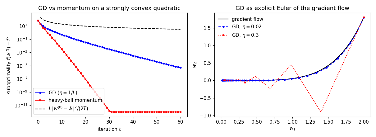
gd.png             : preview figure (checking only).

Data generated by pythondemos/gd.py.
"""

import numpy as np
import matplotlib

matplotlib.use("Agg")
import matplotlib.pyplot as plt

from pathlib import Path

OUT_DIR = Path(__file__).parent

rng = np.random.default_rng(42)
report = []


def check(name, ok):
    report.append((name, bool(ok)))
    print(f"  [{'ok' if ok else 'FAIL'}] {name}")


# ----------------------------------------------------------------------
# Strongly convex quadratic: the ERM objective of least-squares
# linear regression, f(w) = (1/m) || X w - y ||^2.
# ----------------------------------------------------------------------
m, d = 200, 20
X = rng.standard_normal((m, d))
# mild anisotropy so the ratio mu/L (and hence the gap between GD
# and momentum) is visible but not pathological.
X *= np.linspace(1.0, 3.0, d)
w_true = rng.standard_normal(d)
y = X @ w_true + 0.1 * rng.standard_normal(m)

A = (2.0 / m) * (X.T @ X)            # curvature matrix of f; its eigenvalues give mu and L
eigs = np.linalg.eigvalsh(A)
L, mu = float(eigs[-1]), float(eigs[0])   # smoothness / strong-convexity
w_hat = np.linalg.solve(X.T @ X, X.T @ y)  # unique minimizer


def f(w):
    return float(np.mean((X @ w - y) ** 2))


def grad(w):
    return (2.0 / m) * (X.T @ (X @ w - y))


f_star = f(w_hat)
w0 = np.zeros(d)
T = 60

# ----------------------------------------------------------------------
On a strongly convex quadratic f(w) = (1/m)||Xw - y||^2 (the ERM objective of least-squares linear regression), the GD step w <- w - eta grad f(w) with eta = 1/L does not increase f at any iteration and converges to the unique minimizer w_hat = argmin f.
# ----------------------------------------------------------------------
eta = 1.0 / L
w = w0.copy()
gd_gap = [f(w) - f_star]
gd_vals = [f(w)]
for _ in range(T):
    w = w - eta * grad(w)
    gd_vals.append(f(w))
    gd_gap.append(f(w) - f_star)

monotone = all(gd_vals[t + 1] <= gd_vals[t] + 1e-12 for t in range(T))
check("[P-descent] GD is monotone non-increasing (eta = 1/L)", monotone)
# "ideally converge to a minimum": the iterate moves toward w_hat and the
# suboptimality shrinks by orders of magnitude over the run.
closer = np.linalg.norm(w - w_hat) < np.linalg.norm(w0 - w_hat)
check("[P-descent] GD iterate moves toward w_hat", closer)
check("[P-descent] GD reduces suboptimality >1e5x", gd_gap[-1] < 1e-5 * gd_gap[0])

# ----------------------------------------------------------------------
  [ok] [P-descent] GD is monotone non-increasing (eta = 1/L)
  [ok] [P-descent] GD iterate moves toward w_hat
  [ok] [P-descent] GD reduces suboptimality >1e5x
For the convex L-smooth objective, the constant step eta=1/L obeys the suboptimality bound f(w^(T)) - f* <= L ||w^(0) - w_hat||^2 / (2 T), i.e. the suboptimality falls in proportion to 1/T.
# ----------------------------------------------------------------------
dist0_sq = float(np.linalg.norm(w0 - w_hat) ** 2)
bound_ok = all(
    gd_gap[t] <= L * dist0_sq / (2.0 * t) + 1e-9 for t in range(1, T + 1)
)
check("[P-rate] f(w^T) - f* <= L||w0-w_hat||^2/(2T) for all T", bound_ok)

# ----------------------------------------------------------------------
[ok] [P-rate] f(w^T) - f* <= L||w0-w_hat||^2/(2T) for all T
Polyak's heavy-ball momentum w^(t+1) = w^(t) - eta grad f(w^(t)) + beta (w^(t) - w^(t-1)), which combines gradients over several steps, reaches a given suboptimality in far fewer iterations than plain GD on the same strongly convex quadratic.
# ----------------------------------------------------------------------
sqL, sqmu = np.sqrt(L), np.sqrt(mu)
eta_hb = 4.0 / (sqL + sqmu) ** 2
beta_hb = ((sqL - sqmu) / (sqL + sqmu)) ** 2
w_prev = w0.copy()
w = w0.copy()
hb_gap = [f(w) - f_star]
for _ in range(T):
    w_next = w - eta_hb * grad(w) + beta_hb * (w - w_prev)
    w_prev, w = w, w_next
    hb_gap.append(f(w) - f_star)

tol = 1e-6
gd_hit = next((t for t, g in enumerate(gd_gap) if g <= tol), None)
hb_hit = next((t for t, g in enumerate(hb_gap) if g <= tol), None)
faster = hb_hit is not None and (gd_hit is None or hb_hit < gd_hit)
check(f"[P-momentum] momentum hits {tol:g} first (hb={hb_hit}, gd={gd_hit})", faster)

# ----------------------------------------------------------------------
[ok] [P-momentum] momentum hits 1e-06 first (hb=18, gd=None)
the GD operator F^(eta): solutions are fixed points;
# non-expansive for eta = 1/L; a contraction with factor 1 - mu*eta under
# mu-strong convexity, so the iterates converge geometrically to the
# unique fixed point (Banach fixed-point theorem).
# ----------------------------------------------------------------------
F = lambda wv: wv - eta * grad(wv)
check("[P-fixedpoint] F(w_hat) = w_hat (solutions are fixed points)",
      np.linalg.norm(F(w_hat) - w_hat) < 1e-10)
pairs = rng.standard_normal((300, 2, d))
ne = all(np.linalg.norm(F(a) - F(b)) <= np.linalg.norm(a - b) + 1e-12
         for a, b in pairs)
check("[P-fixedpoint] F non-expansive for eta = 1/L (300 random pairs)", ne)
kappa = 1.0 - mu * eta
ctr = all(np.linalg.norm(F(a) - F(b)) <= kappa * np.linalg.norm(a - b) + 1e-12
          for a, b in pairs)
check(f"[P-fixedpoint] contraction with factor 1 - mu*eta = {kappa:.4f}", ctr)
wfp = w0.copy()
it_err = [np.linalg.norm(wfp - w_hat)]
for _ in range(T):
    wfp = F(wfp)
    it_err.append(np.linalg.norm(wfp - w_hat))
geo_it = all(it_err[t + 1] <= kappa * it_err[t] + 1e-12 for t in range(T))
check("[P-fixedpoint] ||w^(t+1) - w_hat|| <= (1 - mu*eta) ||w^(t) - w_hat||",
      geo_it)

# ----------------------------------------------------------------------
  [ok] [P-fixedpoint] F(w_hat) = w_hat (solutions are fixed points)
  [ok] [P-fixedpoint] F non-expansive for eta = 1/L (300 random pairs)
  [ok] [P-fixedpoint] contraction with factor 1 - mu*eta = 0.9190
  [ok] [P-fixedpoint] ||w^(t+1) - w_hat|| <= (1 - mu*eta) ||w^(t) - w_hat||
mu-strongly convex geometric bound
# f(w^(t)) - f* <= (1 - mu/L)^t (f(w^(0)) - f*)
# ----------------------------------------------------------------------
geo_bound = all(gd_gap[t] <= (1.0 - mu / L) ** t * gd_gap[0] + 1e-12
                for t in range(T + 1))
check("[P-rate-geo] f(w^t) - f* <= (1 - mu/L)^t (f(w^0) - f*)", geo_bound)

# ----------------------------------------------------------------------
[ok] [P-rate-geo] f(w^t) - f* <= (1 - mu/L)^t (f(w^0) - f*)
Nesterov's accelerated variant of GD obeys the improved
# bound f(w^(T)) - f* <= 2 L ||w^(0) - w_hat||^2 / (T+1)^2.
# ----------------------------------------------------------------------
y_seq = w0.copy()
w_cur = w0.copy()
nes_gap = [f(w_cur) - f_star]
for t in range(1, T + 1):
    w_next = y_seq - (1.0 / L) * grad(y_seq)
    y_seq = w_next + (t - 1.0) / (t + 2.0) * (w_next - w_cur)
    w_cur = w_next
    nes_gap.append(f(w_cur) - f_star)
nes_bound = all(nes_gap[t] <= 2.0 * L * dist0_sq / (t + 1) ** 2 + 1e-9
                for t in range(1, T + 1))
check("[P-nesterov] Nesterov obeys 2L||w0 - w_hat||^2/(T+1)^2", nes_bound)
check("[P-nesterov] Nesterov reaches a smaller gap than plain GD at T",
      nes_gap[-1] < gd_gap[-1])

# ----------------------------------------------------------------------
  [ok] [P-nesterov] Nesterov obeys 2L||w0 - w_hat||^2/(T+1)^2
  [ok] [P-nesterov] Nesterov reaches a smaller gap than plain GD at T
GD is exactly the explicit Euler discretization of the gradient flow dw/dt = -grad f(w): one GD step with step size eta equals one explicit-Euler step of the ODE, and the deviation of the GD iterate from the exact flow trajectory at a fixed time horizon shrinks in proportion to eta (properties of the flow transfer to GD for small eta).
# dw/dt = -grad f(w), on the 2-d quadratic f(w) = (w1^2 + 5 w2^2)/2
# (grad f(w) = A2 w with diagonal A2, so the flow w(t) = exp(-A2 t) w(0) is exact).
# ----------------------------------------------------------------------
A2 = np.diag([1.0, 5.0])
w0_2d = np.array([2.0, 1.8])


def grad2(w):
    return A2 @ w


def flow(t):
    return np.exp(-np.diag(A2) * t) * w0_2d


def euler_step(w, eta):
    return w + eta * (-grad2(w))         # explicit Euler for dw/dt = -grad f


def gd_step(w, eta):
    return w - eta * grad2(w)            # the GD update


# one GD step IS one explicit-Euler step (the identification is exact)
w_probe = rng.standard_normal(2)
check(
    "[P-euler] GD step equals explicit-Euler step of the flow",
    np.allclose(gd_step(w_probe, 0.1), euler_step(w_probe, 0.1)),
)

# global discretization error at fixed horizon tau shrinks like eta
tau = 1.0
errs = {}
for eta2 in (0.1, 0.01):
    k = int(round(tau / eta2))
    w = w0_2d.copy()
    for _ in range(k):
        w = gd_step(w, eta2)
    errs[eta2] = float(np.linalg.norm(w - flow(tau)))
ratio = errs[0.01] / errs[0.1]
check(
    f"[P-euler] error at tau=1 falls ~ eta (ratio {ratio:.3f}, expect ~0.1)",
    ratio < 0.2,
)

# trajectories for the entry's flow figure
with open(OUT_DIR / "gd_flow.csv", "w") as fh:
    fh.write("t,w1,w2\n")
    for t in np.linspace(0.0, 6.0, 300):
        w1, w2 = flow(t)
        fh.write(f"{t:.4f},{w1:.6e},{w2:.6e}\n")

for eta2, steps, name in ((0.02, 250, "small"), (0.3, 14, "large")):
    w = w0_2d.copy()
    with open(OUT_DIR / f"gd_flow{name}.csv", "w") as fh:
        fh.write("k,w1,w2\n")
        fh.write(f"0,{w[0]:.6e},{w[1]:.6e}\n")
        for k in range(1, steps + 1):
            w = gd_step(w, eta2)
            fh.write(f"{k},{w[0]:.6e},{w[1]:.6e}\n")

# ----------------------------------------------------------------------
# CSV for the entry's pgfplots figure (clip tiny values so log axis is
# well-defined).
# ----------------------------------------------------------------------
floor = 1e-12
with open(OUT_DIR / "gd_convergence.csv", "w") as fh:
    fh.write("iter,gd,momentum\n")
    for t in range(T + 1):
        fh.write(f"{t},{max(gd_gap[t], floor):.8e},{max(hb_gap[t], floor):.8e}\n")

# ----------------------------------------------------------------------
# preview figure (checking only)
# ----------------------------------------------------------------------
fig, (ax, ax2) = plt.subplots(1, 2, figsize=(11, 4))
it = np.arange(T + 1)
ax.semilogy(it, np.maximum(gd_gap, floor), "b-o", ms=3, label="GD ($\\eta=1/L$)")
ax.semilogy(it, np.maximum(hb_gap, floor), "r-s", ms=3, label="heavy-ball momentum")
ax.semilogy(
    it[1:], L * dist0_sq / (2.0 * it[1:]), "k--", label="$L\\|w^{(0)}-\\hat w\\|^2/(2T)$"
)
ax.set_xlabel("iteration $t$")
ax.set_ylabel("suboptimality $f(w^{(t)})-f^\\star$")
ax.legend()
ax.set_title("GD vs momentum on a strongly convex quadratic")

ts = np.linspace(0.0, 6.0, 300)
fl = np.array([flow(t) for t in ts])
ax2.plot(fl[:, 0], fl[:, 1], "k-", label="gradient flow")
for eta2, steps, style, lab in (
    (0.02, 250, "b--o", "GD, $\\eta=0.02$"),
    (0.3, 14, "r:s", "GD, $\\eta=0.3$"),
):
    w = w0_2d.copy()
    traj = [w.copy()]
    for _ in range(steps):
        w = gd_step(w, eta2)
        traj.append(w.copy())
    traj = np.array(traj)
    ax2.plot(traj[:, 0], traj[:, 1], style, ms=3, markevery=5, label=lab)
ax2.set_xlabel("$w_1$")
ax2.set_ylabel("$w_2$")
ax2.legend(frameon=False)
ax2.set_title("GD as explicit Euler of the gradient flow")
fig.tight_layout()
fig.savefig(OUT_DIR / "gd.png", dpi=110)

print(f"\nL={L:.3f}, mu={mu:.3f}, cond={L/mu:.1f}")
ok = all(v for _, v in report)
print("ALL OK" if ok else "SOME CHECKS FAILED")
  [ok] [P-euler] GD step equals explicit-Euler step of the flow
  [ok] [P-euler] error at tau=1 falls ~ eta (ratio 0.100, expect ~0.1)

L=21.015, mu=1.703, cond=12.3
ALL OK
P-euler writes when the script runs