P-algos writes when the script runsDictionary of Applied Machine Learning · hypothesis space
Numerical companion to the entry hypothesis space: it recomputes what the entry states and prints one line per check
One block per paragraph of the entry (marked [P...]): each block verifies numerically what the corresponding statement asserts. Self-contained (numpy/matplotlib only), fixed seed.
Run it without installing anything:uv run https://dictionaryofml.org/terms/hypospace.py
uv downloads this script and the pinned NumPy and Matplotlib it needs, then runs it; the script fetches any input file it uses. To keep the output files, download hypospace.py into a folder and run uv run hypospace.py there. With NumPy and Matplotlib already installed, python3 hypospace.py, from any directory — it writes its output files into the current directory. Fixed seeds, so the printed numbers reproduce exactly. Download hypospace.py · Notebook · Open in Colab
One cell per block of the script: the code, and what that code printed when it last ran here
"""
hypospace.py — numerical companion to the glossary entry
'hypothesis space'.

One block per paragraph of the entry (marked [P...]): each block verifies
numerically what the corresponding statement asserts. Self-contained
(numpy/matplotlib only), fixed seed.

Blocks
------
[P-def]      The hypothesis space is the committed set of candidate maps,
             a subset of Y^X: for |X| = 4, |Y| = 2 the full map space has
             16 elements, the threshold subset only 5.
[P-examples] Canonical hypothesis spaces: the linear model (linear maps
             R^d -> R closed under evaluation) and the set of maps
             realizable by a fixed ANN architecture as its parameters
             vary (different parameters, different maps; same
             architecture).
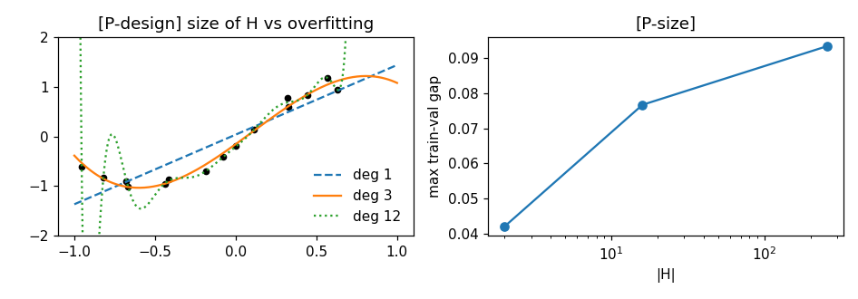
[P-design]   The choice of H trades computation against the number of
             data points: with m = 15 points, raising the polynomial
             degree (larger H) drives the error on the trainset down but
             the error on fresh data points up — the overfitting limit on
             the usable size of H.
[P-size]     The size of H anticipates generalization BEFORE training:
             the maximal generalization gap over H grows with the
             cardinality |H| (finite classes of random threshold maps).
[P-algos]    The same H serves different algorithms: ERM on a fixed
             training set, online learning over a stream, and Bayesian inference (a
             posterior over a finite H) all operate on one linear
             hypothesis space; ERM and online learning agree in the limit,
             the posterior concentrates on the same hypothesis.

Outputs
-------
hypospace.png : preview figure (checking only).

Data generated by pythondemos/hypospace.py.
"""

import numpy as np
import matplotlib

matplotlib.use("Agg")
import matplotlib.pyplot as plt
from pathlib import Path

OUT_DIR = Path(__file__).parent

from itertools import product

rng = np.random.default_rng(42)
report = []


def check(name, ok):
    report.append((name, bool(ok)))
    print(f"  [{'ok' if ok else 'FAIL'}] {name}")
The hypothesis space is the committed set of candidate maps, a subset of Y^X: for |X| = 4, |Y| = 2 the full map space has 16 elements, the threshold subset only 5.
print("[P-def] H is a subset of Y^X")
X_space, Y_space = [0, 1, 2, 3], [0, 1]
all_maps = set(product(Y_space, repeat=4))
H_thresh = {tuple(int(x >= t) for x in X_space) for t in range(5)}
check("|Y^X| = 16", len(all_maps) == 16)
check("H (threshold maps) is a strict subset of Y^X",
      H_thresh < all_maps)
[P-def] H is a subset of Y^X
  [ok] |Y^X| = 16
  [ok] H (threshold maps) is a strict subset of Y^X
Canonical hypothesis spaces: the linear model (linear maps R^d -> R closed under evaluation) and the set of maps realizable by a fixed ANN architecture as its parameters vary (different parameters, different maps; same architecture).
print("[P-examples] linear model and fixed-architecture ANN as H")
w1, w2 = rng.normal(size=3), rng.normal(size=3)
x = rng.normal(size=3)
check("linear model: every parameter vector w defines the map x -> w^T x",
      np.isclose(w1 @ x, np.sum(w1 * x)))
relu = lambda a: np.maximum(a, 0)
ann = lambda W, v, xx: v @ relu(W @ xx)           # fixed 3-8-1 architecture
W_a, v_a = rng.normal(size=(8, 3)), rng.normal(size=8)
W_b, v_b = rng.normal(size=(8, 3)), rng.normal(size=8)
check("fixed ANN architecture: different parameters realize different maps",
      not np.isclose(ann(W_a, v_a, x), ann(W_b, v_b, x)))
[P-examples] linear model and fixed-architecture ANN as H
  [ok] linear model: every parameter vector w defines the map x -> w^T x
  [ok] fixed ANN architecture: different parameters realize different maps
The choice of H trades computation against the number of data points: with m = 15 points, raising the polynomial degree (larger H) drives the error on the trainset down but the error on fresh data points up — the overfitting limit on the usable size of H.
print("[P-design] larger H overfits a small trainset")
m = 15
xd = np.sort(rng.uniform(-1, 1, m))
yd = np.sin(2.5 * xd) + 0.15 * rng.normal(size=m)
xv = rng.uniform(-1, 1, 200)
yv = np.sin(2.5 * xv) + 0.15 * rng.normal(size=200)
tr_err, va_err = [], []
for deg in (1, 3, 12):
    c = np.polyfit(xd, yd, deg)
    tr_err.append(np.mean((yd - np.polyval(c, xd)) ** 2))
    va_err.append(np.mean((yv - np.polyval(c, xv)) ** 2))
print(f"    train err deg 1,3,12: {tr_err[0]:.3f}, {tr_err[1]:.3f}, "
      f"{tr_err[2]:.4f} | val err: {va_err[0]:.3f}, {va_err[1]:.3f}, "
      f"{va_err[2]:.1f}")
check("the error on the trainset decreases with the size of H",
      tr_err[0] > tr_err[1] > tr_err[2])
check("the error on fresh data points blows up for the largest H (overfitting)",
      va_err[2] > 5 * va_err[1])
[P-design] larger H overfits a small trainset
    train err deg 1,3,12: 0.098, 0.009, 0.0012 | val err: 0.098, 0.043, 58356.0
  [ok] the error on the trainset decreases with the size of H
  [ok] the error on fresh data points blows up for the largest H (overfitting)
The size of H anticipates generalization BEFORE training: the maximal generalization gap over H grows with the cardinality |H| (finite classes of random threshold maps).
print("[P-size] the size of H bounds the gap before training")
mg = 60
xg_tr, xg_va = rng.uniform(0, 1, mg), rng.uniform(0, 1, 1000)
yg_tr = (xg_tr > 0.5).astype(float)
yg_va = (xg_va > 0.5).astype(float)
def max_gap(n_hypos):
    ts = rng.uniform(0, 1, n_hypos)               # random threshold class
    gaps = [abs(np.mean((xg_tr > t) != yg_tr)
                - np.mean((xg_va > t) != yg_va)) for t in ts]
    return max(gaps)
gaps = [np.mean([max_gap(n) for _ in range(30)]) for n in (2, 16, 256)]
print(f"    max train-val gap for |H| = 2, 16, 256: "
      f"{gaps[0]:.3f}, {gaps[1]:.3f}, {gaps[2]:.3f}")
check("the maximal gap over H grows with |H|", gaps[0] < gaps[1] < gaps[2])
[P-size] the size of H bounds the gap before training
    max train-val gap for |H| = 2, 16, 256: 0.028, 0.054, 0.071
  [ok] the maximal gap over H grows with |H|
The same H serves different algorithms: ERM on a fixed training set, online learning over a stream, and Bayesian inference (a posterior over a finite H) all operate on one linear hypothesis space; ERM and online learning agree in the limit, the posterior concentrates on the same hypothesis.
print("[P-algos] one H, three algorithms")
mt = 200
Xa = rng.normal(size=(mt, 2))
w_true = np.array([1.0, -0.5])
ya = Xa @ w_true + 0.1 * rng.normal(size=mt)
w_erm = np.linalg.lstsq(Xa, ya, rcond=None)[0]    # ERM on a fixed training set
w_og = np.zeros(2)                                # online learning on the stream
for t in range(mt):
    w_og += 0.05 * (ya[t] - w_og @ Xa[t]) * Xa[t]
H_fin = [w_true, np.array([0.0, 0.0]), np.array([-1.0, 0.5]),
         np.array([1.0, 0.5])]                    # finite H for Bayes
log_post = np.array([-np.sum((ya - Xa @ w) ** 2) / (2 * 0.1**2)
                     for w in H_fin])
post = np.exp(log_post - log_post.max())
post /= post.sum()
check("ERM on a fixed trainset and online learning agree on the same H "
      "(|w| close)",
      np.linalg.norm(w_erm - w_og) < 0.1)
check("Bayesian inference returns a distribution over H that "
      "concentrates on the best hypothesis",
      post[0] > 0.99)

# ------------------------------------------------------------ preview
fig, ax = plt.subplots(1, 2, figsize=(8.6, 3.0))
xx = np.linspace(-1, 1, 300)
ax[0].plot(xd, yd, "ko", ms=4)
for deg, st in ((1, "--"), (3, "-"), (12, ":")):
    ax[0].plot(xx, np.polyval(np.polyfit(xd, yd, deg), xx), st,
               label=f"deg {deg}")
ax[0].set_ylim(-2, 2); ax[0].legend(frameon=False)
ax[0].set_xlabel("feature $x$"); ax[0].set_ylabel("label $y$")
ax[0].set_title("[P-design] size of H vs overfitting")
ax[1].semilogx([2, 16, 256], gaps, "o-")
ax[1].set_xlabel("|H|"); ax[1].set_ylabel("max generalization gap")
ax[1].set_title("[P-size]")
fig.tight_layout()
fig.savefig(OUT_DIR / "hypospace.png", dpi=110)
print(f"\n{sum(ok for _, ok in report)}/{len(report)} checks passed")
assert all(ok for _, ok in report)
[P-algos] one H, three algorithms
  [ok] ERM on a fixed trainset and online learning agree on the same H (|w| close)
  [ok] Bayesian inference returns a distribution over H that concentrates on the best hypothesis

9/9 checks passed
P-algos writes when the script runs