B-plot writes when the script runsDictionary of Applied Machine Learning · feature learning
Numerical companion to the entry feature learning: it recomputes what the entry states and prints one line per check
Numerical companion to the glossary entry 'featlearn' (feature learning). The GeoSphere Austria weather station Krems (station id 3805) records eight daily measurements: minimum, maximum and mean air temperature, precipitation, sunshine duration, relative humidity, air pressure and wind speed. This script downloads the records for 2024 from the GeoSphere data hub (dataset klima-v2-1d) and writes them to featlearn_weather.csv. A value of -1 for precipitation marks a trace of rain too small to record and is set to 0.
Run it with python3 featlearn.py, from any directory — it writes its output files into the current directory. Requires NumPy and Matplotlib only, and uses fixed seeds, so the printed numbers reproduce exactly. Download featlearn.py · Notebook · Open in Colab
One cell per block of the script: the code, and what that code printed when it last ran here
"""Feature learning on a year of weather at Krems: forty raw measurements
of the previous five days become two learned features, and a linear
model on the two features predicts the next day's maximum temperature.

Purpose
-------
Numerical companion to the glossary entry 'featlearn' (feature learning).
The GeoSphere Austria weather station Krems (station id 3805) records
eight daily measurements: minimum, maximum and mean air temperature,
precipitation, sunshine duration, relative humidity, air pressure and
wind speed.  This script downloads the records for 2024 from the
GeoSphere data hub (dataset klima-v2-1d) and writes them to
featlearn_weather.csv.  A value of -1 for precipitation marks a trace
of rain too small to record and is set to 0.

Each day from January 6 to December 31 is a data point.  Its label is
the maximum temperature of that day; its raw features are the eight
measurements of each of the five previous days, a list of forty
numbers.  A day cannot be drawn as a point with forty coordinates, so
the demo learns a feature transformation that delivers two new
features: principal component analysis (PCA) on the forty raw features,
each scaled to zero sample mean and unit sample variance because
temperatures, precipitation and pressure carry different units.  The
demo checks the entry's claims: the PCA transformation has the minimum
linear reconstruction error, equal to the sum of the dropped eigenvalues
of the sample covariance matrix; the two learned features are the
coordinates of a scatterplot in which warm and cold days separate,
most of each class on its own side of the first feature's zero; and
linear regression on the two learned features predicts the label on
held-out days far better than the sample mean of the training labels.

Deterministic: the data are a fixed archive year, PCA is an eigenvalue
decomposition, and the random linear transformations used for
comparison are drawn with a fixed seed.  Self-contained: numpy +
matplotlib only (stdlib urllib for the download).

Blocks
------
[B-fetch] Download the eight daily measurements at Krems for 2024 and
          write them to featlearn_weather.csv; check the count and one
          pinned value against the archive.
[B-dataset] Build the 361 data points: forty raw features (five previous
          days times eight measurements) and the label (maximum
          temperature of the day); scale every raw feature to zero
          sample mean and unit sample variance.
[B-pca] Learn the feature transformation: the two eigenvectors of the
          sample covariance matrix with the largest eigenvalues; check
          the reconstruction-error identity, that no random linear
          transformation reconstructs better, and that warm and cold
          days separate along the first learned feature.
[B-linreg] Fit linear regression to the two learned features on the
          days of January to August and validate on September to
          December; compare with the forty raw features and with the
          sample mean of the training labels.
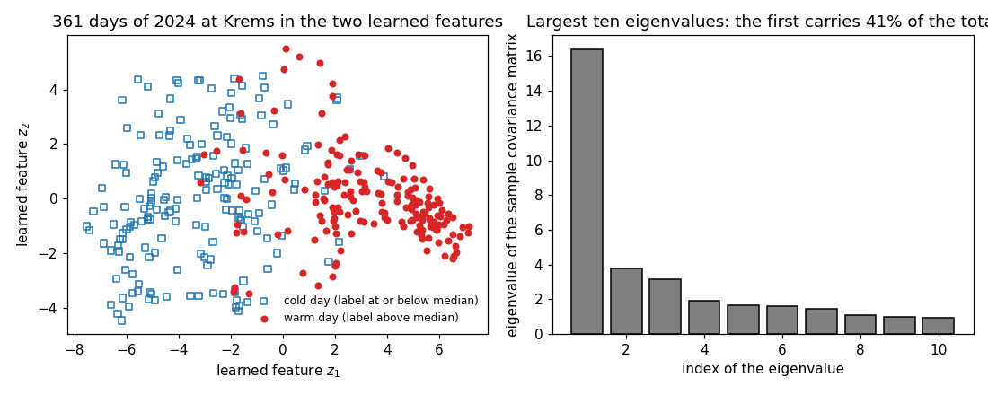
[B-plot] Preview: the scatterplot of the days in the two learned
          features, warm and cold days marked differently, and the
          largest ten eigenvalues of the sample covariance matrix (the
          first is 16.4 of a total of 40, i.e., 41 percent).

Outputs
-------
featlearn_weather.csv   : date and the eight measurements, 366 days of 2024
featlearn_warm.csv      : z1, z2 of the days whose label is above the median
featlearn_cold.csv      : z1, z2 of the days whose label is at or below it
featlearn_eigvals.csv   : index, eigenvalue of the sample covariance matrix
featlearn_valerr.csv    : model, validation error (mean squared error)
featlearn.png           : preview (checking only)
"""

import json
import urllib.request
from pathlib import Path

import numpy as np
import matplotlib

matplotlib.use("Agg")
import matplotlib.pyplot as plt

OUT_DIR = Path(__file__).parent

report = []                         # collects (check name, pass/fail) pairs


def check(name, ok):                # records and prints one verification
    report.append((name, bool(ok)))
    print(f"  [{'ok' if ok else 'FAIL'}] {name}")
Download the eight daily measurements at Krems for 2024 and write them to featlearn_weather.csv; check the count and one pinned value against the archive.
PARAMS = ["tlmin", "tlmax", "tl_mittel", "rr", "so_h", "rf_mittel",
          "p_mittel", "vv_mittel"]
URL = ("https://dataset.api.hub.geosphere.at/v1/station/historical/"
       f"klima-v2-1d?parameters={','.join(PARAMS)}&station_ids=3805"
       "&start=2024-01-01&end=2024-12-31")
with urllib.request.urlopen(URL, timeout=120) as resp:
    payload = json.load(resp)
params = payload["features"][0]["properties"]["parameters"]
stamps = [t[:10] for t in payload["timestamps"]]
M = np.stack([np.array(params[p]["data"], dtype=float) for p in PARAMS], 1)
M[:, 3] = np.maximum(M[:, 3], 0.0)          # -1 marks a trace of rain
with open(OUT_DIR / "featlearn_weather.csv", "w") as f:
    f.write("date," + ",".join(PARAMS) + "\n")
    for day, row in zip(stamps, M):
        f.write(day + "," + ",".join(f"{v:g}" for v in row) + "\n")
check("[B-fetch] 366 days with eight measurements downloaded for 2024",
      M.shape == (366, 8))
check("[B-fetch] the record matches the archive (Feb 1: -3.8 to 10.4 deg)",
      stamps[31] == "2024-02-01" and np.allclose(M[31, :2], [-3.8, 10.4]))
  [ok] [B-fetch] 366 days with eight measurements downloaded for 2024
  [ok] [B-fetch] the record matches the archive (Feb 1: -3.8 to 10.4 deg)
Build the 361 data points: forty raw features (five previous days times eight measurements) and the label (maximum temperature of the day); scale every raw feature to zero sample mean and unit sample variance.
LAG = 5
days = np.arange(LAG, len(M))                       # Jan 6 .. Dec 31
X_raw = np.stack([M[t - LAG:t].ravel() for t in days])   # 361 x 40
y = M[days, 1]                                      # tlmax of the day
m, d = X_raw.shape
mu, sigma = X_raw.mean(axis=0), X_raw.std(axis=0)
X = (X_raw - mu) / sigma                            # zero mean, unit variance
check("[B-dataset] 361 data points with forty raw features each",
      (m, d) == (361, 40))
check("[B-dataset] every scaled feature has unit sample variance",
      np.allclose(X.var(axis=0), 1.0))
  [ok] [B-dataset] 361 data points with forty raw features each
  [ok] [B-dataset] every scaled feature has unit sample variance
  eigenvalues 1-3: 16.39, 3.78, 3.13 of total 40
  reconstruction error PCA 7159, best of 20 random transformations 8338
Learn the feature transformation: the two eigenvectors of the sample covariance matrix with the largest eigenvalues; check the reconstruction-error identity, that no random linear transformation reconstructs better, and that warm and cold days separate along the first learned feature.
Q = X.T @ X / m                                     # sample covariance matrix
eigvals, eigvecs = np.linalg.eigh(Q)
order = np.argsort(eigvals)[::-1]
eigvals, eigvecs = eigvals[order], eigvecs[:, order]
W = eigvecs[:, :2].T                                # 2 x 40
Z = X @ W.T                                         # z = W x, 361 x 2


def reconstruction_error(W):
    """Minimum over R of sum_r ||x^(r) - R W x^(r)||^2 (least squares)."""
    Zc = X @ W.T
    R = np.linalg.lstsq(Zc, X, rcond=None)[0].T     # d x 2
    return float(((X - Zc @ R.T) ** 2).sum())


err_pca = reconstruction_error(W)
rng = np.random.default_rng(0)
err_random = [reconstruction_error(rng.standard_normal((2, d)))
              for _ in range(20)]
print(f"  eigenvalues 1-3: {eigvals[0]:.2f}, {eigvals[1]:.2f}, "
      f"{eigvals[2]:.2f} of total {eigvals.sum():.0f}")
print(f"  reconstruction error PCA {err_pca:.0f}, best of 20 random "
      f"transformations {min(err_random):.0f}")
check("[B-pca] the reconstruction error equals m times the sum of the "
      "dropped eigenvalues", np.isclose(err_pca, m * eigvals[2:].sum()))
check("[B-pca] no random linear transformation reconstructs better",
      err_pca < min(err_random))
warm = y > np.median(y)
frac_warm = float((Z[warm, 0] > 0).mean())      # warm days right of z1 = 0
frac_cold = float((Z[~warm, 0] <= 0).mean())    # cold days left of it
print(f"  first learned feature positive for {100 * frac_warm:.0f}% of the "
      f"warm days, nonpositive for {100 * frac_cold:.0f}% of the cold days")
check("[B-pca] warm and cold days separate along the first learned feature "
      "(at least 85% of each class on its side of z1 = 0)",
      min(frac_warm, frac_cold) >= 0.85)
np.savetxt(OUT_DIR / "featlearn_warm.csv", Z[warm], delimiter=",",
           header="z1,z2", comments="", fmt="%.3f")
np.savetxt(OUT_DIR / "featlearn_cold.csv", Z[~warm], delimiter=",",
           header="z1,z2", comments="", fmt="%.3f")
np.savetxt(OUT_DIR / "featlearn_eigvals.csv",
           np.stack([np.arange(1, d + 1), eigvals], 1), delimiter=",",
           header="index,eigenvalue", comments="", fmt=["%d", "%.4f"])
  [ok] [B-pca] the reconstruction error equals m times the sum of the dropped eigenvalues
  [ok] [B-pca] no random linear transformation reconstructs better
  first learned feature positive for 89% of the warm days, nonpositive for 92% of the cold days
  [ok] [B-pca] warm and cold days separate along the first learned feature (at least 85% of each class on its side of z1 = 0)
  validation error two learned features: 13.52
  validation error forty raw features: 10.21
  validation error sample mean of training labels: 110.86
Fit linear regression to the two learned features on the days of January to August and validate on September to December; compare with the forty raw features and with the sample mean of the training labels.
train = days < 244                                  # Jan 6 .. Aug 31
val = ~train                                        # Sep 1 .. Dec 31


def linreg_valerr(F):
    """Least squares with intercept on the training days; validation MSE."""
    A = np.hstack([F, np.ones((m, 1))])
    w = np.linalg.lstsq(A[train], y[train], rcond=None)[0]
    return float(((A[val] @ w - y[val]) ** 2).mean())


valerr = {"two learned features": linreg_valerr(Z),
          "forty raw features": linreg_valerr(X),
          "sample mean of training labels":
              float(((y[train].mean() - y[val]) ** 2).mean())}
with open(OUT_DIR / "featlearn_valerr.csv", "w") as f:
    f.write("model,valerr\n")
    for name, e in valerr.items():
        f.write(f"{name},{e:.2f}\n")
        print(f"  validation error {name}: {e:.2f}")
check("[B-linreg] two learned features beat the sample mean of the labels",
      valerr["two learned features"] < valerr["sample mean of training labels"] / 2)
check("[B-linreg] forty raw features are not more than twice as good",
      valerr["forty raw features"] > valerr["two learned features"] / 2)
  [ok] [B-linreg] two learned features beat the sample mean of the labels
  [ok] [B-linreg] forty raw features are not more than twice as good

9/9 checks passed
Preview: the scatterplot of the days in the two learned features, warm and cold days marked differently, and the largest ten eigenvalues of the sample covariance matrix (the first is 16.4 of a total of 40, i.e., 41 percent).
fig, (ax1, ax2) = plt.subplots(1, 2, figsize=(10, 4))
ax1.scatter(Z[~warm, 0], Z[~warm, 1], marker="s", facecolors="none",
            edgecolors="tab:blue", s=22, label="cold day (label at or below median)")
ax1.scatter(Z[warm, 0], Z[warm, 1], marker="o", color="tab:red", s=18,
            label="warm day (label above median)")
ax1.set_xlabel("learned feature $z_1$")
ax1.set_ylabel("learned feature $z_2$")
ax1.set_title("361 days of 2024 at Krems in the two learned features")
ax1.legend(frameon=False, fontsize=8)
ax2.bar(np.arange(1, 11), eigvals[:10], color="0.5", edgecolor="black")
ax2.set_xlabel("index of the eigenvalue")
ax2.set_ylabel("eigenvalue of the sample covariance matrix")
ax2.set_title("Largest ten eigenvalues: the first carries 41% of the total")
fig.tight_layout()
fig.savefig(OUT_DIR / "featlearn.png", dpi=110)

print()
failed = [n for n, ok in report if not ok]
print(f"{len(report) - len(failed)}/{len(report)} checks passed"
      + (f"; FAILED: {failed}" if failed else ""))
B-plot writes when the script runs