pythondemos/linclass.pyDictionary of Applied Machine Learning
Updated on 2026-10-10
See also binary classification logistic regression support vector machine empirical risk minimization
A linear classifier is a classifier whose decision regions are separated by hyperplanes. For binary classification it predicts the sign of a linear model hypothesis $\hypothesis(\featurevec) = \weights^{\top} \featurevec + \offset$, whose decision boundary is the hyperplane with normal vector $\weights$. The hypothesis value $\hypothesis(\featurevec)$ is the distance of $\featurevec$ from that hyperplane, multiplied by $\normgeneric{\weights}{2}$, and its sign names the side. That distance bounds the feature perturbations the prediction tolerates. The model parameters are learned by empirical risk minimization (ERM) with a convex surrogate for the $0/1$ loss: logistic regression uses the logistic loss and the support vector machine (SVM) the hinge loss. More than two label values are handled by one linear model hypothesis per value and the largest-score rule, which makes every decision region an intersection of halfspaces.
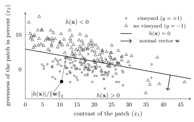
B-fitMapping the vineyards of a wine
region starts from an aerial photograph. The photograph is cut into
square patches of $25$ m side length, and each patch becomes a
data point. Two numbers describe a patch: its contrast
$\feature_{1}$, the standard deviation of the brightness of its pixels,
and its greenness $\feature_{2}$, the relative difference between
the average green and the average red channel value, in percent.
The two numbers form the feature vector
$\featurevec = (\feature_{1}, \feature_{2})^{\top} \in \reals^{2}$,
and the label is $\truelabel = +1$ for a patch showing a
vineyard and $\truelabel = -1$ otherwise. Vine rows alternate
foliage with bare soil, so a vineyard patch is more contrasted and
less green than the forest and meadow around it. A straight line
separates most of the vineyard patches from the rest
(Fig. 1).
pythondemos/linclass.py
The number $\hypothesis(\featurevec)$ carries more than its sign. Consider a feature vector $\featurevec$ and any vector $\featurevec'$ of the decision boundary. Subtracting $\weights^{\top} \featurevec' + \offset = 0$ from $\hypothesis(\featurevec)$ gives \[ \hypothesis(\featurevec) = \weights^{\top} \big( \featurevec - \featurevec' \big) \text{.} \] The Cauchy-Schwarz inequality bounds the right-hand side in magnitude by $\normgeneric{\weights}{2} \normgeneric{\featurevec - \featurevec'}{2}$. Every vector of the decision boundary is therefore at distance at least $|\hypothesis(\featurevec)| / \normgeneric{\weights}{2}$ from $\featurevec$. That distance is attained by the orthogonal projection \[ \featurevec' = \featurevec - \frac{\hypothesis(\featurevec)} {\normgeneric{\weights}{2}^{2}} \, \weights \text{,} \] which satisfies $\weights^{\top} \featurevec' + \offset = 0$. The distance of $\featurevec$ from the decision boundary is thus $|\hypothesis(\featurevec)| / \normgeneric{\weights}{2}$, and the hypothesis value $\hypothesis(\featurevec)$ is that distance multiplied by $\normgeneric{\weights}{2}$, with the sign naming the side (Bishop, 2006, Sect. 4.1.1; Hastie et al., 2009, Sect. 4.5, Eq. (4.40)). Fig. 1 shows this distance for one vineyard patch.
B-scaleThe hypothesis value by itself does not measure that distance. Let $s$ be a positive number. Replacing the model parameters $(\weights, \offset)$ by $(s \weights, s \offset)$ leaves the decision boundary and every prediction unchanged, while every hypothesis value is multiplied by $s$. Dividing by $\normgeneric{\weights}{2}$ removes this freedom, which is why the distance and not $\hypothesis(\featurevec)$ is the quantity with a geometric meaning.
B-robustThe distance also bounds the feature perturbations that a prediction tolerates. Perturbing $\featurevec$ by a vector $\boldsymbol{\delta}$ changes the hypothesis value by $\weights^{\top} \boldsymbol{\delta}$, which the Cauchy-Schwarz inequality bounds in magnitude by $\normgeneric{\weights}{2} \normgeneric{\boldsymbol{\delta}}{2}$. The sign of $\hypothesis(\featurevec)$, and with it the prediction, therefore survives every perturbation with $\normgeneric{\boldsymbol{\delta}}{2} < |\hypothesis(\featurevec)| / \normgeneric{\weights}{2}$. A vineyard patch far from the decision boundary keeps its prediction under a measurement error that flips the prediction for a patch close to it. Multiplying $\hypothesis(\featurevec)$ by the label $\truelabel$ gives the margin, which is positive exactly on the correctly classified data points. For a linearly separable training set and a sufficiently small regularization parameter $\regparam$, the support vector machine (SVM) learns the linear classifier whose smallest margin is largest (Shalev-Shwartz and Ben-David, 2014, Sect. 15.1, Eq. (15.1)).
The model parameters $(\weights, \offset)$ are learned from a training set $\trainset = \{ (\featurevec^{(\sampleidx)}, \truelabel^{(\sampleidx)}) \}_{\sampleidx = 1}^{\samplesize}$ by empirical risk minimization (ERM). Counting the mistakes with the $0/1$ loss gives an objective function that is piecewise constant, and minimizing it is computationally hard outside the linearly separable case (Shalev-Shwartz and Ben-David, 2014, Sect. 9.1). Practical methods replace the $0/1$ loss by a convex loss of the margin: logistic regression uses the logistic loss and the SVM uses the hinge loss. Both learn a hypothesis from the same hypothesis space, the linear model, and differ only in the loss. Both objective functions are convex: gradient descent (GD) minimizes the smooth one of logistic regression, and subgradient descent with a subgradient the non-smooth one of the SVM. Adding a penalty term $\regparam \normgeneric{\weights}{2}^{2}$ to the average loss, one of the three routes that regularization distinguishes, keeps $\normgeneric{\weights}{2}$ small and the margins wide (Shalev-Shwartz and Ben-David, 2014, Sect. 15.2).
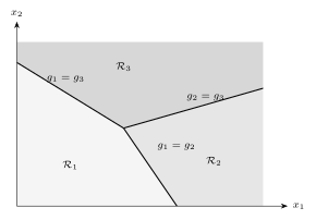
For more than two label values, with $\labelspace = \{1,
\ldots, \nrcategories\}$, a linear classifier uses one
linear model hypothesis
$g_{\clusteridx}(\featurevec) = \big( \weights^{(\clusteridx)}
\big)^{\top} \featurevec + \offset^{(\clusteridx)}$ per
label value $\clusteridx \in \labelspace$ and predicts the
value with the largest score,
$\predictedlabel = \argmax_{\clusteridx \in \labelspace}
g_{\clusteridx}(\featurevec)$. The decision region
$\decreg{\clusteridx}$ is then an intersection of
$\nrcategories - 1$ halfspaces, one per competing
label value, and is therefore a convex set; the border
between $\decreg{\clusteridx}$ and $\decreg{\clusteridx'}$ lies in
the hyperplane on which the two scores agree
(Bishop, 2006, Sect. 4.1.2, Eq. (4.10)). The resulting
partition of the feature space is shown in
Fig. 2.
See also: classifier, binary classification, decision boundary, decision region, hyperplane, halfspace, linear model, margin, logistic regression, support vector machine, empirical risk minimization, $\bf 0/1$ loss, feature transformation.
@misc{dictml_linclass,
  author = {Jung, Alexander},
  editor = {Olioumtsevits, Konstantina and Schnoor, Ekkehard},
  title = {linear classifier},
  howpublished = {Dictionary of Applied Machine Learning (course edition)},
  year = {2026},
  doi = {10.5281/zenodo.21569296},
  note = {ISBN 978-952-64-3013-3, CC BY 4.0, retrieved 2026-10-10},
  url = {https://dictionaryofml.org/terms/linclass.html}
}