B-preview writes when the script runsDictionary of Applied Machine Learning · linear classifier
Numerical companion to the entry linear classifier: it recomputes what the entry states and prints one line per check
A binary classification trainset for the vineyard task: each data point is a square patch of an aerial photograph, described by two numeric features — the contrast of the patch (the standard deviation of its pixel brightness) and its greenness (the relative difference between the average green and the average red channel value, in percent) — and labelled +1 if the patch shows a vineyard and -1 otherwise. The feature vectors are drawn from a two-component Gaussian model whose means and covariance matrices are the patch statistics measured on an orthophoto of the Wachau valley in Austria (basemap.at, CC BY 4.0; 41,472 patches of 32 x 32 pixels at 0.79 m per pixel, 21 percent of them vineyard). Vine rows alternate foliage with bare soil, which makes a vineyard patch less green and more contrasted than the forest and meadow around it.
Run it without installing anything:uv run https://dictionaryofml.org/terms/linclass.py
uv downloads this script and the pinned NumPy and Matplotlib it needs, then runs it; the script fetches any input file it uses. To keep the output files, download linclass.py into a folder and run uv run linclass.py there. With NumPy and Matplotlib already installed, python3 linclass.py, from any directory — it writes its output files into the current directory. Fixed seeds, so the printed numbers reproduce exactly. Download linclass.py · Notebook · Open in Colab
One cell per block of the script: the code, and what that code printed when it last ran here
"""
linclass.py — numerical companion to the glossary entry 'linear classifier'.

Purpose
-------
A binary classification trainset for the vineyard task: each data point is
a square patch of an aerial photograph, described by two numeric features —
the contrast of the patch (the standard deviation of its pixel brightness)
and its greenness (the relative difference between the average green and
the average red channel value, in percent) — and labelled +1 if the patch
shows a vineyard and -1 otherwise.  The feature vectors are drawn from a
two-component Gaussian model whose means and covariance matrices are the
patch statistics measured on an orthophoto of the Wachau valley in Austria
(basemap.at, CC BY 4.0; 41,472 patches of 32 x 32 pixels at 0.79 m per
pixel, 21 percent of them vineyard).  Vine rows alternate foliage with
bare soil, which makes a vineyard patch less green and more contrasted
than the forest and meadow around it.

A linear classifier is learned from the trainset by gradient descent on
the average logistic loss, and the geometry of its decision boundary is
then checked numerically: the distance of a feature vector from the
decision boundary equals |h(x)| / ||w||; the hypothesis value h(x) alone
does not measure that distance, since rescaling the parameters multiplies
it by the scale factor while leaving the classifier and the distances
unchanged; and a feature perturbation shorter than that distance never
changes the predicted label.  Self-contained (numpy/matplotlib only),
fixed seed.

Blocks
------
[B-patches] m = 240 data points, 120 per class, drawn from the two-
            component model; the contrast is kept positive by redrawing.
            Written to linclass_vineyard.csv and linclass_other.csv for
            the entry's scatter plot.
[B-fit]     The parameters (w, b) of the linear classifier h(x) = w^T x + b
            learned by gradient descent on the average logistic loss (in
            standardized coordinates, mapped back to the original feature
            units).  The learned classifier beats the constant rule that
            always answers with the majority label.  Its decision boundary
            and its normal vector w go to linclass_boundary.csv and
            linclass_normal.csv.
[B-geom]    The distance of each of the 240 feature vectors from the
            decision boundary, obtained by minimizing the Euclidean
            distance over a fine grid of points of the boundary, agrees
            with |h(x)| / ||w|| to four decimals.  The foot of the
            perpendicular from one marked data point goes to
            linclass_drop.csv.
[B-scale]   Rescaling the parameters, (w, b) -> (c w, c b) with c = 7,
            multiplies every hypothesis value by c but leaves every
            prediction and every distance unchanged: h(x) by itself is
            not a distance, h(x) / ||w|| is.
[B-robust]  Perturbing a feature vector by a vector shorter than its
            distance from the decision boundary never changes the
            predicted label; a perturbation longer than that distance
            can change it.
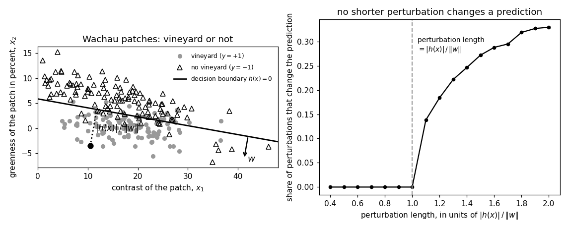
[B-preview] The matplotlib preview of the scatter plot and of the share
            of random perturbations that change a prediction, against
            the perturbation length.

Outputs
-------
linclass_vineyard.csv : x1,x2 — the 120 patches labelled +1 (vineyard).
linclass_other.csv    : x1,x2 — the 120 patches labelled -1.
linclass_boundary.csv : x1,x2 — two endpoints of the decision boundary line.
linclass_normal.csv   : x1,x2 — base and tip of the normal-vector w arrow.
linclass_drop.csv     : x1,x2 — the marked data point and the foot of its
                        perpendicular on the decision boundary.
linclass.png          : matplotlib preview of the figures (checking only).
"""

from pathlib import Path

import numpy as np
import matplotlib

matplotlib.use("Agg")
import matplotlib.pyplot as plt

OUT_DIR = Path(__file__).parent

report = []


def check(name, ok):
    report.append((name, bool(ok)))
    print(f"  [{'ok' if ok else 'FAIL'}] {name}")


def sigmoid(z):
    return 1.0 / (1.0 + np.exp(-z))
240 patches, 120 of each class; contrast in [1.0, 46.1], greenness in [-6.8, 15.2]
m = 240 data points, 120 per class, drawn from the two- component model; the contrast is kept positive by redrawing. Written to linclass_vineyard.csv and linclass_other.csv for the entry's scatter plot.
# mean and covariance of (contrast, greenness) over the patches of the
# orthophoto, by class; vineyard patches are more contrasted and less green
MEAN = {1: np.array([18.16, 0.04]), -1: np.array([14.81, 6.39])}
COV = {1: np.array([[38.46, -3.04], [-3.04, 4.06]]),
       -1: np.array([[99.44, -29.64], [-29.64, 15.84]])}
M_PER_CLASS = 120
rng = np.random.default_rng(4)


def draw(label, n):
    """n feature vectors of one class; the contrast is a standard deviation,
    so a draw with a negative first feature is replaced."""
    out = []
    while len(out) < n:
        z = rng.multivariate_normal(MEAN[label], COV[label])
        if z[0] > 0.0:
            out.append(z)
    return np.array(out)


Xpos, Xneg = draw(1, M_PER_CLASS), draw(-1, M_PER_CLASS)
X = np.r_[Xpos, Xneg]
y = np.r_[np.ones(M_PER_CLASS), -np.ones(M_PER_CLASS)]
m = len(X)
print(f"    {m} patches, {M_PER_CLASS} of each class; "
      f"contrast in [{X[:, 0].min():.1f}, {X[:, 0].max():.1f}], "
      f"greenness in [{X[:, 1].min():.1f}, {X[:, 1].max():.1f}]")
check("[B-patches] 240 data points with two features each",
      X.shape == (240, 2) and len(y) == 240)
check("[B-patches] every contrast is positive", (X[:, 0] > 0.0).all())
check("[B-patches] the vineyard patches are less green on average",
      Xpos[:, 1].mean() < Xneg[:, 1].mean())
for fname, Xc in [("linclass_vineyard.csv", Xpos), ("linclass_other.csv", Xneg)]:
    with open(OUT_DIR / fname, "w") as f:
        f.write("x1,x2\n")
        for a, b_ in Xc:
            f.write(f"{a:.4f},{b_:.4f}\n")
  [ok] [B-patches] 240 data points with two features each
  [ok] [B-patches] every contrast is positive
  [ok] [B-patches] the vineyard patches are less green on average
    w = (-0.150, -0.838), b = 4.912; correctly classified 0.858 against 0.500
The parameters (w, b) of the linear classifier h(x) = w^T x + b learned by gradient descent on the average logistic loss (in standardized coordinates, mapped back to the original feature units). The learned classifier beats the constant rule that always answers with the majority label. Its decision boundary and its normal vector w go to linclass_boundary.csv and linclass_normal.csv.
mu, sd = X.mean(axis=0), X.std(axis=0)
Z = np.c_[(X - mu) / sd, np.ones(m)]      # standardized, constant feature last


def grad(wz):
    return -(Z * (y * sigmoid(-y * (Z @ wz)))[:, None]).mean(axis=0)


wz = np.zeros(3)
for _ in range(6000):
    wz = wz - 0.5 * grad(wz)
weights = wz[:2] / sd                             # w in the original units
offset = float(wz[2] - np.sum(wz[:2] * mu / sd))  # b in the original units
wnorm = float(np.linalg.norm(weights))


def hyp(pts):
    return np.atleast_1d(pts @ weights + offset)


acc = float(np.mean(np.sign(hyp(X)) == y))
acc_const = float(max((y > 0).mean(), (y < 0).mean()))
print(f"    w = ({weights[0]:.3f}, {weights[1]:.3f}), b = {offset:.3f}; "
      f"correctly classified {acc:.3f} against {acc_const:.3f}")
check("[B-fit]     the learned classifier beats the constant majority rule",
      acc > acc_const)
check("[B-fit]     the gradient has (almost) vanished",
      float(np.linalg.norm(grad(wz))) < 1e-3)

X1LO, X1HI = 0.0, 48.0                            # the plotted range of x1


def x2_on_boundary(x1):
    return -(weights[0] * x1 + offset) / weights[1]


with open(OUT_DIR / "linclass_boundary.csv", "w") as f:
    f.write("x1,x2\n")
    for x1 in (X1LO, X1HI):
        f.write(f"{x1:.4f},{x2_on_boundary(x1):.4f}\n")

# the normal vector w, drawn from a point of the boundary into the half-space
# that the classifier labels +1 (where h is positive)
unit_w = weights / wnorm
base = np.array([42.0, x2_on_boundary(42.0)])
ARROW = 4.5                                       # arrow length in feature units
tip = base + ARROW * unit_w
check("[B-fit]     the arrow points into the half-space labelled +1",
      float(hyp(tip)[0]) > 0.0)
with open(OUT_DIR / "linclass_normal.csv", "w") as f:
    f.write("x1,x2\n")
    for pt in (base, tip):
        f.write(f"{pt[0]:.4f},{pt[1]:.4f}\n")
  [ok] [B-fit]     the learned classifier beats the constant majority rule
  [ok] [B-fit]     the gradient has (almost) vanished
  [ok] [B-fit]     the arrow points into the half-space labelled +1
    largest deviation between |h(x)|/||w|| and the grid search: 1.67e-05
The distance of each of the 240 feature vectors from the decision boundary, obtained by minimizing the Euclidean distance over a fine grid of points of the boundary, agrees with |h(x)| / ||w|| to four decimals. The foot of the perpendicular from one marked data point goes to linclass_drop.csv.
dist_formula = np.abs(hyp(X)) / wnorm
# the same distance, obtained by searching a fine grid of boundary points
t = np.linspace(-400.0, 400.0, 400001)
along = np.array([-weights[1], weights[0]]) / wnorm      # unit vector, w^T . = 0
foot0 = -offset * weights / (weights @ weights)          # a point of the boundary
line = foot0 + t[:, None] * along
dist_grid = np.array([np.min(np.linalg.norm(line - x, axis=1)) for x in X])
gap = float(np.abs(dist_grid - dist_formula).max())
print(f"    largest deviation between |h(x)|/||w|| and the grid search: {gap:.2e}")
check("[B-geom]    |h(x)|/||w|| is the distance from the decision boundary",
      gap < 1e-4)
# a vineyard patch on the sparse left flank of the cloud, as far from the
# decision boundary as the plot can show without the drop crossing the clouds
left = (X[:, 0] > 5.0) & (X[:, 0] < 12.0)
left[M_PER_CLASS:] = False                        # vineyard patches only
MARK = int(np.argmax(np.where(left, dist_formula, -np.inf)))
x_mark = X[MARK]
foot = x_mark - float(hyp(x_mark)[0]) / (weights @ weights) * weights
print(f"    marked patch ({x_mark[0]:.2f}, {x_mark[1]:.2f}): h(x) = "
      f"{float(hyp(x_mark)[0]):.2f}, |h(x)|/||w|| = {dist_formula[MARK]:.2f}")
check("[B-geom]    the foot of the perpendicular lies on the boundary",
      abs(float(hyp(foot)[0])) < 1e-9)
check("[B-geom]    the drop from the marked patch is orthogonal to the boundary",
      abs(float((x_mark - foot) @ along)) < 1e-9)
with open(OUT_DIR / "linclass_drop.csv", "w") as f:
    f.write("x1,x2\n")
    for pt in (x_mark, foot):
        f.write(f"{pt[0]:.4f},{pt[1]:.4f}\n")
  [ok] [B-geom]    |h(x)|/||w|| is the distance from the decision boundary
    marked patch (10.51, -3.52): h(x) = 6.29, |h(x)|/||w|| = 7.39
  [ok] [B-geom]    the foot of the perpendicular lies on the boundary
  [ok] [B-geom]    the drop from the marked patch is orthogonal to the boundary
Rescaling the parameters, (w, b) -> (c w, c b) with c = 7, multiplies every hypothesis value by c but leaves every prediction and every distance unchanged: h(x) by itself is not a distance, h(x) / ||w|| is.
C = 7.0
h_scaled = C * hyp(X)
dist_scaled = np.abs(h_scaled) / (C * wnorm)
check("[B-scale]   rescaling multiplies every hypothesis value by c",
      np.allclose(h_scaled, C * hyp(X)) and abs(C - 1.0) > 0.5)
check("[B-scale]   rescaling leaves every prediction unchanged",
      np.array_equal(np.sign(h_scaled), np.sign(hyp(X))))
check("[B-scale]   rescaling leaves every distance unchanged",
      np.allclose(dist_scaled, dist_formula))
  [ok] [B-scale]   rescaling multiplies every hypothesis value by c
  [ok] [B-scale]   rescaling leaves every prediction unchanged
  [ok] [B-scale]   rescaling leaves every distance unchanged
    4800 perturbations of each length: 0 shorter ones and 217 longer ones change the prediction
Perturbing a feature vector by a vector shorter than its distance from the decision boundary never changes the predicted label; a perturbation longer than that distance can change it.
n_short = n_flip_short = n_flip_long = 0
for idx in range(m):
    for _ in range(20):
        direction = rng.normal(size=2)
        direction /= np.linalg.norm(direction)
        short = direction * (0.99 * dist_formula[idx])
        long_ = direction * (1.01 * dist_formula[idx])
        n_short += 1
        n_flip_short += int(np.sign(hyp(X[idx] + short)[0]) != np.sign(hyp(X[idx])[0]))
        n_flip_long += int(np.sign(hyp(X[idx] + long_)[0]) != np.sign(hyp(X[idx])[0]))
print(f"    {n_short} perturbations of each length: {n_flip_short} shorter ones "
      f"and {n_flip_long} longer ones change the prediction")
check("[B-robust]  no perturbation shorter than the distance changes a prediction",
      n_flip_short == 0)
check("[B-robust]  some perturbation longer than the distance does change one",
      n_flip_long > 0)
  [ok] [B-robust]  no perturbation shorter than the distance changes a prediction
  [ok] [B-robust]  some perturbation longer than the distance does change one

14/14 checks pass
wrote linclass_vineyard.csv, linclass_other.csv, linclass_boundary.csv, linclass_normal.csv, linclass_drop.csv, linclass.png in /Users/junga1/dictionaryappliedml/pythondemos
The matplotlib preview of the scatter plot and of the share of random perturbations that change a prediction, against the perturbation length.
fig, (ax, ax2) = plt.subplots(1, 2, figsize=(10.4, 4.2))
ax.plot(Xpos[:, 0], Xpos[:, 1], "o", color="0.6", ms=5,
        label="vineyard ($y = +1$)")
ax.plot(Xneg[:, 0], Xneg[:, 1], "^", color="black", mfc="none", ms=6,
        label="no vineyard ($y = -1$)")
ax.plot([X1LO, X1HI], [x2_on_boundary(X1LO), x2_on_boundary(X1HI)], "k-",
        lw=1.8, label="decision boundary $h(x) = 0$")
ax.annotate("", xy=tuple(tip), xytext=tuple(base),
            arrowprops=dict(arrowstyle="->", lw=1.6))
ax.text(tip[0] + 0.6, tip[1] - 0.6, "$w$", fontsize=12)
ax.plot([x_mark[0], foot[0]], [x_mark[1], foot[1]], "k:", lw=1.8)
ax.plot(*x_mark, "o", color="black", ms=7)
ax.text(x_mark[0] + 1.0, 0.5 * (x_mark[1] + foot[1]) - 0.6,
        "$|h(x)|\\,/\\,\\|w\\|$", fontsize=11)
ax.set_xlim(X1LO, X1HI)
ax.set_aspect("equal")
ax.set_xlabel("contrast of the patch, $x_1$")
ax.set_ylabel("greenness of the patch in percent, $x_2$")
ax.set_title("Wachau patches: vineyard or not")
ax.legend(frameon=False, fontsize=8, loc="upper right")
radii = np.linspace(0.4, 2.0, 17)
flipped = []
for r in radii:
    d_rand = rng.normal(size=(m, 40, 2))
    d_rand /= np.linalg.norm(d_rand, axis=2, keepdims=True)
    moved = X[:, None, :] + d_rand * (r * dist_formula)[:, None, None]
    flipped.append(float(np.mean(np.sign(moved @ weights + offset)
                                 != np.sign(hyp(X))[:, None])))
ax2.plot(radii, flipped, "o-", color="black", ms=4)
ax2.axvline(1.0, color="0.6", ls="--", lw=1.4)
ax2.text(1.04, 0.28, "perturbation length\n$= |h(x)|\\,/\\,\\|w\\|$", fontsize=9)
ax2.set_xlabel("perturbation length, in units of $|h(x)|\\,/\\,\\|w\\|$")
ax2.set_ylabel("share of perturbations that change the prediction")
ax2.set_title("no shorter perturbation changes a prediction")
fig.tight_layout()
fig.savefig(OUT_DIR / "linclass.png", dpi=110)

n_ok = sum(ok for _, ok in report)
print(f"\n{n_ok}/{len(report)} checks pass")
print(f"wrote linclass_vineyard.csv, linclass_other.csv, linclass_boundary.csv, "
      f"linclass_normal.csv, linclass_drop.csv, linclass.png in {OUT_DIR}")
if n_ok != len(report):
    raise SystemExit(1)
B-preview writes when the script runs