Dictionary of Applied Machine Learning
Updated on 2026-09-30
Typeset PDF version — the authoritative form of this entry
Binary classification is the machine learning (ML) problem of predicting which of two labels a data point carries, from its features. The label space holds two elements, written either $\{-1, +1\}$ or $\{0, 1\}$; the margin-based loss functions assume the first convention. A classifier partitions the feature space into two decision regions separated by a decision boundary, which is a hyperplane for a linear classifier. The natural loss function is the $0/1$ loss, whose average over a dataset is $1$ minus the accuracy, but it is not convex in the model parameters, so practical methods minimize a convex surrogate that upper bounds it: the logistic loss for logistic regression, the hinge loss for the support vector machine (SVM). Because the two kinds of mistake usually carry different costs, the confusion matrix is reported beside the accuracy.
A weather service that answers whether the maximum temperature of the coming day will reach $25$ degrees Celsius returns one of two answers, yes or no, and nothing in between. The same shape of question is asked of an email (spam or not), of a credit application (default or not) and of a biopsy image (malignant or benign). Binary classification is the machine learning (ML) problem behind all of them: predict which of two labels a data point carries, from its features.
Binary classification is classification with a
label space $\labelspace$ that holds two elements. The two
elements are usually written $\labelspace = \{-1, +1\}$ or
$\labelspace = \{0, 1\}$. The choice is a convention and not a
modelling decision, but it must be fixed before a loss function is
written down: the logistic loss and the hinge loss are defined
through the margin $\truelabel \cdot \hypothesis(\featurevec)$ and
therefore assume $\{-1, +1\}$. A
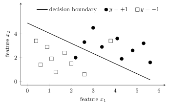
classifier is a hypothesis $\hypothesis: \featurespace
\rightarrow \labelspace$, and it partitions the feature space
into two decision regions, one per label, separated by
a decision boundary. For a linear classifier the
decision boundary is a hyperplane $\weights^{\top}
\featurevec + \weight_{0} = 0$, and the label predicted for
$\featurevec$ is the side of that hyperplane on which
$\featurevec$ lies (Bishop, 2006, Sect. 4.1.1). A data point
that lands on the side of the other label is misclassified and
incurs a $0/1$ loss of $1$ (Fig. 1).
A single number is a thin summary of a binary classifier. The two kinds of mistake, a wrong yes and a wrong no, generally carry different costs, and on imbalanced data the accuracy of the constant answer is already high (baseline). Both are reasons to report the confusion matrix, and the precision, recall and F$_1$ score computed from it, beside the accuracy.
For example, a spam filter reads the features of an email and returns $\truelabel = +1$ for spam and $\truelabel = -1$ for legitimate mail. A wrong $+1$ hides a legitimate email from the user while a wrong $-1$ only delivers one more piece of spam, so the two mistakes are not interchangeable and the classifier is tuned to keep the first rare.
Synonyms: two-class classification.
See also: classification, classifier, decision boundary, $\bf 0/1$ loss, logistic loss, logistic regression, accuracy, confusion matrix, imbalanced data, baseline.
@misc{dictml_binclass,
  author = {Jung, Alexander},
  editor = {Olioumtsevits, Konstantina and Schnoor, Ekkehard},
  title = {binary classification},
  howpublished = {Dictionary of Applied Machine Learning (course edition)},
  year = {2026},
  doi = {10.5281/zenodo.21569296},
  note = {ISBN 978-952-64-3013-3, CC BY 4.0, retrieved 2026-09-30},
  url = {https://dictionaryofml.org/terms/binclass.html}
}