featuretransformation.py, which recomputes what the entry states: the script block by block · open in ColabDictionary of Applied Machine Learning: 147 machine-learning terms, each with a definition, a figure, citations and a Python demo · All terms · Demos · Start here
Updated on 2026-11-20
Readiness 90/100
See also feature learning feature feature space principal component analysis linear discriminant analysis random projection autoencoder dimensionality reduction kernel method regularization hyperparameter decision tree
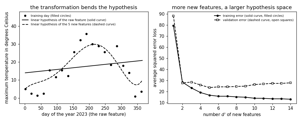
A feature transformation is a function that maps the feature vector of a data point to a new feature vector, so that a machine learning (ML) method runs on the new features in place of the raw ones. What is learned is then the composition of the transformation with a hypothesis on the new feature space, which is why a linear model of the new features is not a linear model of the raw ones. Methods differ in where the transformation comes from: principal component analysis (PCA) obtains it from the raw features alone, linear discriminant analysis (LDA) uses the labels as well, a random projection draws it at random, and an autoencoder learns it with an artificial neural network (ANN). Each hidden layer of a deep net is one more feature transformation, and a kernel method fixes one through the choice of a kernel without ever evaluating it. The number of new features sizes the hypothesis space of the method that runs on them, so keeping it small is model pruning, one of the three routes that regularization distinguishes. For the maximum daytime temperature at Krems an der Donau (Austria), the first five powers of the day of the year turn a nearly flat hypothesis into a curve that follows the seasons and cut the validation error from $88.2$ to $23.6$ squared degrees. The choice matters as much as the count: the three odd powers of the day leave the validation error above that of the constant hypothesis, which is why the transformation is often learned from the dataset rather than chosen by hand.
featuretransformation.py, which recomputes what the entry states: the script block by block · open in ColabB-rawA weather station at Krems
an der Donau (Austria) records the maximum daytime temperature of
every day of $2023$ and $2024$. Each day is a data point, its
label is that temperature, and its single raw feature
$x$ is the position of the day in the year, rescaled to the
interval $[-1, 1]$. The $365$ days of $2023$ form the
training set $\mathcal{D}^{(\rm train)}$ and the $366$ days of $2024$ the
validation set $\mathcal{D}^{(\rm val)}$. Linear regression on $x$ learns a
nearly flat hypothesis from $\mathcal{D}^{(\rm train)}$ by
least squares: it rises by $6.9$ degrees from the first day
of the year to the last, against a label range of $38.4$
degrees. Its training error is $79.4$ squared degrees and its
validation error $88.2$, above the $84.9$ of the constant
hypothesis that always predicts the sample mean of the
labels in $\mathcal{D}^{(\rm train)}$. Replacing $x$ by the five
numbers $x, x^{2}, \ldots, x^{5}$ and running
the same method on them gives a curve that follows the seasons,
with a validation error of $23.6$.
Fig. 1(a) draws the two learned
hypotheses over the days of $\mathcal{D}^{(\rm train)}$.
pythondemos/featuretransformation.py
Methods differ in where ${\mathbf \Phi}$ comes from. Principal component analysis (PCA) obtains it from the raw features alone, as the linear map of a given rank whose reconstruction error is smallest (Hastie et al., 2009, Sect. 14.5.1). Linear discriminant analysis (LDA) uses the labels as well, projecting onto the subspace spanned by the class centroids (Hastie et al., 2009, Sect. 4.3.3). A random projection draws ${\mathbf \Phi}$ at random instead of learning it (Johnson and Lindenstrauss, 1984), and an autoencoder learns a nonlinear ${\mathbf \Phi}$ with an artificial neural network (ANN) (Hinton and Salakhutdinov, 2006). Each hidden layer of a deep net is one more feature transformation, learned jointly with the output layer (Mallat, 2016). A kernel method fixes ${\mathbf \Phi}$ through the choice of a kernel, which returns the inner product of two transformed feature vectors (Schölkopf and Smola, 2002, Sect. 1.1). Such a method uses the transformed feature vectors only through those inner products, so ${\mathbf \Phi}$ is never evaluated (Schölkopf and Smola, 2002, Sect. 1.5). A transformation that delivers fewer new features than the data point has raw ones is dimensionality reduction, and obtaining ${\mathbf \Phi}$ from a dataset rather than by hand is the subject of feature learning.
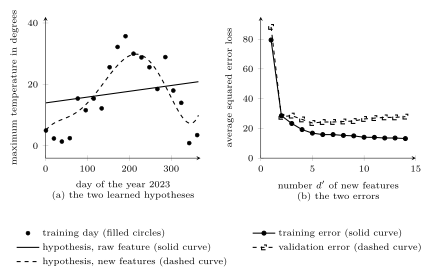
B-pruneThe number $d'$ of new features in the definition \(\eqref{equ_feattrafo_def_dict}\) sizes the hypothesis space of the method that runs on them. For the powers \(\eqref{equ_feattrafo_poly_dict}\), every hypothesis available at $d'$ is available at $d' + 1$ as well, so the training error, the average squared error loss over $\mathcal{D}^{(\rm train)}$, cannot rise with $d'$: it falls from $79.4$ to $13.2$ squared degrees as $d'$ grows from $1$ to $14$. The validation error on $\mathcal{D}^{(\rm val)}$ behaves differently. It is smallest at $d' = 5$ with $23.6$ squared degrees and rises again to $27.9$ at $d' = 14$, the overfitting that a large hypothesis space brings (Bishop, 2006, Sect. 1.1). Fig. 1(b) draws the two errors. Keeping $d'$ small therefore shrinks the hypothesis space, which is model pruning, one of the three routes that regularization distinguishes.
Two other names are in use for the function \(\eqref{equ_feattrafo_def_dict}\). The kernel method literature calls it a feature map (Schölkopf and Smola, 2002, Sect. 2.1), and the statistical learning literature a basis expansion (Hastie et al., 2009, Sect. 5.1). The two senses of feature map are distinct: a feature transformation is the map between feature spaces of the definition \(\eqref{equ_feattrafo_def_dict}\), while a feature map is the grid of activations delivered by one channel of a convolutional layer.
B-blindSince the training error cannot rise with $d'$, it cannot report the cost of a transformation that delivers too many new features, so $d'$ is a hyperparameter and is chosen on held-out data points by validation. The count is not the whole choice, since a transformation fixed before the labels are looked at can discard what the label depends on. The three odd powers $x, x^{3}, x^{5}$ leave the validation error at $86.7$ squared degrees, above the $84.9$ of the constant hypothesis, while the two even powers $x^{2}, x^{4}$ alone give $22.0$. Every odd power is antisymmetric about $x = 0$, the middle of the year, and the maximum daytime temperature at Krems is nearly symmetric about that point. The composition \(\eqref{equ_feattrafo_comp_dict}\) also changes what a weight means: a weight of a linear model on the new features multiplies one of them, at Krems a cube of a rescaled calendar position, and not a quantity the station recorded.
In return, least squares on the new features reaches hypotheses that no linear model of the raw feature contains, at Krems a curve that follows the seasons where a straight line is of no use. Two alternatives avoid the choice of ${\mathbf \Phi}$ by hand. One keeps the raw features and takes a method whose hypothesis space is not a linear model of them, such as a decision tree. The other obtains ${\mathbf \Phi}$ from the dataset, which is feature learning, with an autoencoder or the hidden layers of a deep net.
Synonyms: feature map, basis expansion.
See also: feature learning, feature, feature space, principal component analysis, linear discriminant analysis, random projection, autoencoder, dimensionality reduction, kernel method, feature map, polynomial regression, regularization, hyperparameter, validation, decision tree.
@misc{dictml_featuretransformation,
  author = {Jung, Alexander},
  editor = {Olioumtsevits, Konstantina and Schnoor, Ekkehard},
  title = {feature transformation},
  howpublished = {Dictionary of Applied Machine Learning (course edition)},
  year = {2026},
  doi = {10.5281/zenodo.21569296},
  note = {ISBN 978-952-64-3013-3, CC BY 4.0, retrieved 2026-11-20},
  url = {https://dictionaryofml.org/terms/featuretransformation.html}
}