sqerrloss.py, which recomputes what the entry states: the script block by block · open in ColabDictionary of Applied Machine Learning: 147 machine-learning terms, each with a definition, a figure, citations and a Python demo · All terms · Demos · Start here
Updated on 2026-11-19
Readiness 88/100
See also loss logistic loss $\bf 0/1$ loss training error mean squared error empirical risk minimization linear regression gradient descent maximum likelihood Gaussian random variable outlier clustering error
The squared error loss of a hypothesis on a data point with a numeric label is the square of the difference between the label and the prediction that the hypothesis delivers for the features of the data point. Its average over a training set is the training error, also called the mean squared error (MSE), and minimizing that average over a linear model is least squares, whose solution the normal equations give in closed form. Up to an increasing affine transformation, the squared error loss is the negative log-likelihood function of the label under Gaussian noise around the prediction, so least squares is maximum likelihood estimation. The hypothesis with the smallest risk under the squared error loss is the conditional expectation of the label given the features, and the risk of any other hypothesis exceeds it by the expected squared difference from that conditional expectation. The squared error loss is convex and differentiable in the prediction with a slope proportional to the error, so a single outlier moves the learned hypothesis in proportion to its error, while the absolute error loss and the Huber loss bound that displacement.
sqerrloss.py, which recomputes what the entry states: the script block by block · open in ColabB-dataA weather service predicts the maximum daytime temperature at Krems an der Donau from the morning minimum of the same day. Each day is a data point with the feature $x$, the morning minimum, and the label $y \in \mathbb{R}$, the maximum. A hypothesis $h$ delivers the prediction $\widehat{y} = h(x)$, and the maximum measured in the afternoon says by how many degrees that prediction was off. For a data point with feature vector ${\mathbf x} \in \mathcal{X}$ and numeric label $y \in \mathbb{R}$, consider a hypothesis $h: \mathcal{X} \rightarrow \mathbb{R}$. The squared error loss it incurs is the square of the difference between the label and its prediction (Hastie et al., 2009, Sect. 2.4), \begin{equation} \label{equ_sqerrloss_def_dict} L\left(\left( {\mathbf x},y \right),h \right) := \big(y - h({\mathbf x})\big)^{2} \text{.} \end{equation}
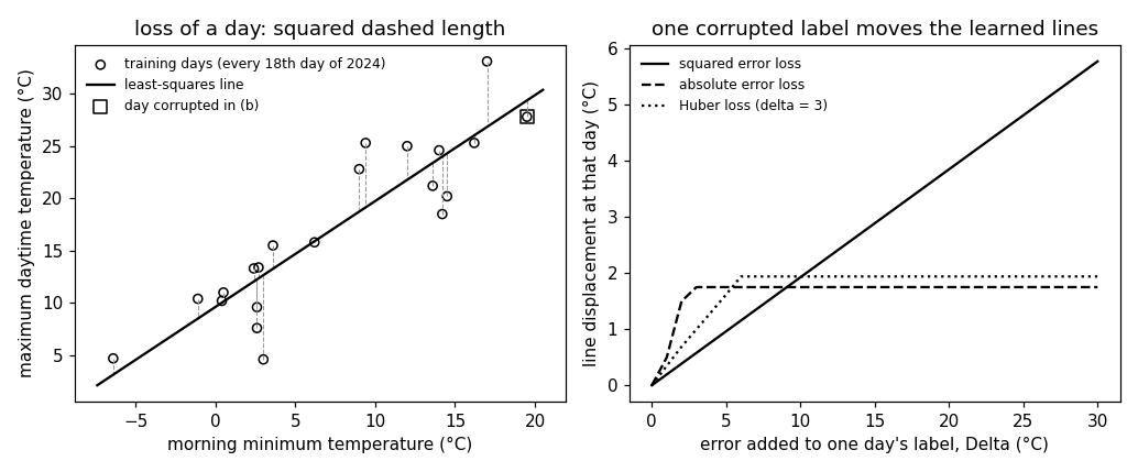
On 8 December 2024 the morning minimum at Krems was $3.0$ degrees and the maximum $4.6$ degrees. The linear hypothesis $\widehat{h}(x) = 9.62 + 1.01 x$ learned below predicts $12.66$ degrees for that morning, so its squared error loss \(\eqref{equ_sqerrloss_def_dict}\) on that day is $(4.6 - 12.66)^{2} \approx 65.0$ squared degrees. The squared error loss is measured in the squared unit of the label, vanishes exactly when the prediction is correct, and is the same for a prediction too high as for one too low by the same amount.
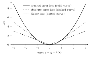
B-lossAs a function of the prediction $\widehat{y}$, the
squared error loss \(\eqref{equ_sqerrloss_def_dict}\) is a parabola
with its minimum at $\widehat{y} = y$, as
Fig. 1 shows. It is convex and
differentiable, with derivative $-2(y -
\widehat{y})$: its slope grows in proportion to the error. For
a linear model $h({\mathbf x}) = {\mathbf w}^{\top}
{\mathbf x}$, the squared error loss is a convex and
differentiable function of the model parameters
${\mathbf w}$ as well, which is what makes gradient descent (GD) applicable. The
absolute error loss $|y - \widehat{y}|$ is convex too
but non-smooth at $\widehat{y} = y$, and its
slope is $\pm 1$ whatever the size of the error. The
Huber loss with threshold $\delta > 0$ is quadratic for a
small error and linear for a large one
(Hastie et al., 2009, Eq. (10.23)). In terms of the
error $e := y - h({\mathbf x})$, it is
\begin{equation}
\label{equ_sqerrloss_huber_dict}
\begin{cases}
e^{2} & \text{for } |e| \leq \delta \text{,} \\
2 \delta |e| - \delta^{2} & \text{otherwise} \text{,}
\end{cases}
\end{equation}
so it agrees with the squared error loss for an error up to
$\delta$ and its slope is capped at $2 \delta$ beyond
(Huber, 1992).
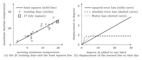
B-constantTake as training set every $18$th day of $2024$ at Krems, $21$ days, with the constant feature $1$ appended to the morning minimum so that $\widehat{{\mathbf w}}$ holds an intercept and a slope. The closed form \(\eqref{equ_sqerrloss_closedform_dict}\) gives the line $\widehat{h}(x) = 9.62 + 1.01 x$ of Fig. 2(a), with training error $12.75$ squared degrees, or $3.57$ degrees after taking the root. The best constant prediction under the squared error loss is the sample mean of the labels, $17.14$ degrees, and its training error is their sample variance, $62.05$: the average squared error of a constant $c$ is that variance plus $(c - 17.14)^{2}$. Under the absolute error loss the best constant is the median of the labels instead, $15.80$ degrees.
B-gaussThe squared error loss is the loss behind maximum likelihood estimation when the label is modeled as the prediction plus Gaussian noise. Let $y = h({\mathbf x}) + \varepsilon$ with a Gaussian random variable (Gaussian RV) $\varepsilon$ of mean zero and variance $\sigma^{2}$, so that $y$ given ${\mathbf x}$ has the probability density function (pdf) $\mathcal{N}\left(h({\mathbf x}),\sigma^{2}\right)$. The negative logarithm of that pdf at the observed label is (Bishop, 2006, Sect. 3.1.1, Eqs. (3.11)–(3.12)) \begin{equation} \label{equ_sqerrloss_nll_dict} - \ln \mathcal{N}\left(h({\mathbf x}),\sigma^{2}\right) (y) = \frac{1}{2 \sigma^{2}} \big(y - h({\mathbf x})\big)^{2} + \frac{1}{2} \ln \big(2 \pi \sigma^{2}\big) \text{,} \end{equation} an increasing affine function of the squared error loss \(\eqref{equ_sqerrloss_def_dict}\). For data points that are realizations of independent and identically distributed (i.i.d.) random variables (RVs), the negative log-likelihood function of the training set is the sum of the terms \(\eqref{equ_sqerrloss_nll_dict}\) over its data points, which is $m / (2 \sigma^{2})$ times the training error \(\eqref{equ_sqerrloss_trainerr_dict}\) plus a constant. The maximum likelihood estimate of ${\mathbf w}$ is therefore the least squares solution \(\eqref{equ_sqerrloss_closedform_dict}\), whatever $\sigma^{2}$ is, and the maximum likelihood estimate of $\sigma^{2}$ is the training error itself, $12.75$ for the $21$ days. The logistic loss is the negative log-likelihood function for a binary label, and Laplacian instead of Gaussian noise gives the absolute error loss (Murphy, 2012, Sect. 7.4).
The risk of a hypothesis is its expected loss under a probabilistic model with a joint probability distribution $\mathbb{P}^{({\mathbf x}, y)}$ of the feature vector and the label. Under the squared error loss, the risk is minimized by the conditional expectation $h^{*}({\mathbf x}) = \mathbb{E}\{y \mid {\mathbf x}\}$, the Bayes estimator for this loss (Bishop, 2006, Sect. 1.5.5, Eq. (1.89); Hastie et al., 2009, Sect. 2.4, Eq. (2.13)). The risk of any hypothesis $h$ splits into two parts (Bishop, 2006, Eq. (1.90)), \begin{equation} \label{equ_sqerrloss_risk_dict} \mathbb{E}\big\{\big(y - h({\mathbf x})\big)^{2}\big\} = \mathbb{E}\big\{\big(h^{*}({\mathbf x}) - h({\mathbf x})\big)^{2}\big\} + \mathbb{E}\big\{\big(y - h^{*}({\mathbf x})\big)^{2}\big\} \text{,} \end{equation} the expected squared difference between $h$ and the conditional expectation, and the expected conditional variance of the label, which no hypothesis can reduce. For a hypothesis learned from a random training set, the first part of the decomposition \(\eqref{equ_sqerrloss_risk_dict}\) splits further into the squared bias and the variance of the learned prediction, the decomposition behind the bias–variance trade-off (Hastie et al., 2009, Sect. 7.3, Eq. (7.9)). Under the absolute error loss the Bayes estimator is the conditional median (Hastie et al., 2009, Eq. (2.18)). The two constant predictions above are the training set versions of these two facts, with the average over the $21$ days in place of the expectation.
The growing slope of the parabola has a cost. A data point whose label is far from the prediction enters the gradient of the training error \(\eqref{equ_sqerrloss_trainerr_dict}\) in proportion to its error, so an outlier pulls the learned hypothesis toward itself without bound (Hastie et al., 2009, Sect. 10.6). For least squares the pull is explicit. Adding $\Delta$ to the label of the $r$th training day changes the solution \(\eqref{equ_sqerrloss_closedform_dict}\) by $({\mathbf X}^{\top} {\mathbf X})^{-1} {\mathbf x}^{(r)} \Delta$. The prediction for that day changes by $\ell_{r} \Delta$, where $\ell_{r} = ({\mathbf x}^{(r)})^{\top} ({\mathbf X}^{\top} {\mathbf X})^{-1} {\mathbf x}^{(r)}$ is the leverage of the day.
B-outlierAmong the $21$ days, the one with the warmest morning, 17 July 2024
with minimum $19.5$ and maximum $27.8$ degrees, has leverage
$0.192$. Each degree added to its label moves the
least squares line at that morning by $0.192$ degrees, which
is $5.76$ degrees for $\Delta = 30$, and the slope of the line
rises from $1.01$ to $1.37$ (Fig. 2(b),
solid curve). Under the absolute error loss, whose ERM solution is
least absolute deviation regression, the line moves by at most $1.75$ degrees, and
not at all once $\Delta$ exceeds $3$ (dashed curve). The
slope of the absolute error loss is $\pm 1$, so once the corrupted day is
above the line, its term in the optimality condition no longer
depends on the size of its error. The Huber loss with $\delta
= 3$ moves its line by $1.93$ degrees and not at all beyond
$\Delta = 6$ (dotted curve), since its slope is capped. This
bounded pull is what robustness to outliers means for
a loss. The absolute error loss is non-smooth, and the
Huber loss adds the threshold $\delta$ as a
hyperparameter; the squared error loss has neither drawback,
and no such bound.
pythondemos/sqerrloss.py
Synonyms: squared loss, quadratic loss.
See also: loss, loss function, absolute error loss, Huber loss, logistic loss, $\bf 0/1$ loss, training error, mean squared error, empirical risk minimization, least squares, linear regression, normal equations, gradient descent, maximum likelihood, Gaussian random variable, risk, Bayes estimator, conditional expectation, bias–variance trade-off, outlier, robustness, least absolute deviation regression, Huber regression, clustering error.
@misc{dictml_sqerrloss,
  author = {Jung, Alexander},
  editor = {Olioumtsevits, Konstantina and Schnoor, Ekkehard},
  title = {squared error loss},
  howpublished = {Dictionary of Applied Machine Learning (course edition)},
  year = {2026},
  doi = {10.5281/zenodo.21569296},
  note = {ISBN 978-952-64-3013-3, CC BY 4.0, retrieved 2026-11-20},
  url = {https://dictionaryofml.org/terms/sqerrloss.html}
}