B-plot writes when the script runsDictionary of Applied Machine Learning · squared error loss
Updated on 2026-11-19
Numerical companion to the entry squared error loss: it recomputes what the entry states and prints one line per check
Numerical companion to the glossary entry 'sqerrloss'. Every 18th day of 2024 at Krems, 21 days, is the training set; a day is a data point whose feature is the morning minimum temperature and whose label the maximum daytime temperature. A hypothesis h(x) = w0 + w1 x predicts the maximum, and the squared error loss of a day is the square of the difference between its label and that prediction.
Run it without installing anything:uv run https://dictionaryofml.org/terms/sqerrloss.py
uv downloads this script and the pinned NumPy and Matplotlib it needs, then runs it; the script fetches any input file it uses. To keep the output files, download sqerrloss.py into a folder and run uv run sqerrloss.py there. With NumPy and Matplotlib already installed, python3 sqerrloss.py, from any directory — it writes its output files into the current directory. Fixed seeds, so the printed numbers reproduce exactly. Download sqerrloss.py · Notebook · Open in Colab
Before running a downloaded copy, scan it: uvx bandit -q -t B102,B307,B602,B605 sqerrloss.py (B102,B307,B602,B605 are the exec, eval and shell checks of bandit) reports nothing: the script runs no shell command and evaluates no generated code.
One cell per block of the script: the code, and what that code printed when it last ran here
"""The squared error loss of a line that predicts the maximum daytime
temperature from the morning minimum at Krems an der Donau.

Purpose
-------
Numerical companion to the glossary entry 'sqerrloss'.  Every 18th day of
2024 at Krems, 21 days, is the training set; a day is a data point whose
feature is the morning minimum temperature and whose label the maximum
daytime temperature.  A hypothesis h(x) = w0 + w1 x predicts the maximum,
and the squared error loss of a day is the square of the difference
between its label and that prediction.

The demo checks the entry's claims: the training error of a hypothesis is
the average of the per-day squared error losses; the least-squares line
solves the normal equations and incurs a smaller average than any other
line; the average squared error of a constant prediction is the sample
variance of the labels plus the squared distance of the constant from
their mean, so the mean is the best constant under the squared error and
the median the best constant under the absolute error; the negative
log-likelihood of a label under Gaussian noise around h(x) is an
increasing affine function of the squared error loss, so least squares is
maximum likelihood; and a single corrupted label moves the least-squares
line in proportion to the corruption while the least-absolute-deviation
and the Huber line stop moving once the corrupted day is far from them.

Deterministic: the training days are a fixed stride through 2024, every
estimate is a closed form or an exact enumeration, and the Huber line is
an iteratively reweighted least-squares fixed point.  Self-contained:
numpy + matplotlib only; the GeoSphere download falls back to the
committed CSV.

Blocks
------
[B-data]      Download the daily minimum and maximum temperature of 2024
              at Krems (GeoSphere station 3805) or read the committed
              copy; 366 days; every 18th day is the training set, 21 days.
[B-loss]      The least-squares line, the squared error loss of each
              training day, and their average, the training error; the
              normal equations hold at the solution, and every other line
              has a larger average loss.
[B-constant]  Constant predictions: the average squared error of a constant
              c is the sample variance of the labels plus (c - mean)^2,
              so the sample mean is the best constant; the median is the
              best constant under the absolute error.
[B-gauss]     Gaussian noise: the negative log-likelihood of a label is an
              increasing affine function of its squared error loss, so the
              least-squares line is the maximum likelihood estimate, and
              the training error is the maximum likelihood variance.
[B-outlier]   One training day's label is raised by Delta = 0, ..., 30
              degrees; the least-squares line moves in proportion to Delta
              (the proportionality constant is the day's leverage), while
              the least-absolute-deviation line and the Huber line stop
              moving once the corrupted day is far from them.
[B-plot]      CSVs for the figure and the matplotlib preview.

Outputs
-------
sqerrloss_weather.csv      : date, tmin, tmax (committed copy).
sqerrloss_points.csv       : the 21 training days with the least-squares
                             prediction and the squared error loss of each.
sqerrloss_lines.csv        : the least-squares line on a grid of mornings.
sqerrloss_outlier.csv      : displacement of the three learned lines at
                             the corrupted day against Delta.
sqerrloss.png              : matplotlib preview (checking only).
"""

# /// script
# requires-python = ">=3.10"
# dependencies = ["matplotlib==3.10.7", "numpy==2.3.4"]
# ///

import json
import urllib.request
from pathlib import Path

import numpy as np
import matplotlib

matplotlib.use("Agg")
import matplotlib.pyplot as plt

OUT_DIR = Path(__file__).parent

report = []


def check(name, ok):
    report.append((name, bool(ok)))
    print(f"  [{'ok' if ok else 'FAIL'}] {name}")
Download the daily minimum and maximum temperature of 2024 at Krems (GeoSphere station 3805) or read the committed copy; 366 days; every 18th day is the training set, 21 days.
print("[B-data] daily minimum and maximum temperature at Krems, 2024")
URL = ("https://dataset.api.hub.geosphere.at/v1/station/historical/"
       "klima-v2-1d?parameters=tlmin,tlmax&station_ids=3805"
       "&start=2024-01-01&end=2024-12-31")
CSV = OUT_DIR / "sqerrloss_weather.csv"
try:
    with urllib.request.urlopen(URL, timeout=120) as resp:
        payload = json.load(resp)
    params = payload["features"][0]["properties"]["parameters"]
    records = [(stamp[:10], lo, hi)
               for stamp, lo, hi in zip(payload["timestamps"],
                                        params["tlmin"]["data"],
                                        params["tlmax"]["data"])]
    with open(CSV, "w") as fh:
        fh.write("date,tmin,tmax\n")
        for day, lo, hi in records:
            fh.write(f"{day},{lo},{hi}\n")
    print(f"    downloaded {len(records)} days")
except OSError as err:
    print(f"    download failed ({err}); reading the committed CSV")
    rows = CSV.read_text().strip().splitlines()[1:]
    records = [(d, float(a), float(b))
               for d, a, b in (r.split(",") for r in rows)]

check("[B-data] 366 days for 2024", len(records) == 366)
check("[B-data] no day is missing a temperature",
      all(lo is not None and hi is not None for _, lo, hi in records))
STRIDE = 18
idx = np.arange(0, len(records), STRIDE)
dates = [records[i][0] for i in idx]
x = np.array([records[i][1] for i in idx], dtype=float)   # morning minimum
y = np.array([records[i][2] for i in idx], dtype=float)   # daytime maximum
m = len(x)
check(f"[B-data] every {STRIDE}th day of 2024 is a training day: {m} days, "
      f"{dates[0]} to {dates[-1]}", m == 21)
X = np.column_stack([np.ones(m), x])   # constant feature + morning minimum


def line(w, x):
    return w[0] + w[1] * x


def sq_loss(w, x, y):
    """Squared error loss of the line w on each data point."""
    return (y - line(w, x)) ** 2


def abs_loss(w, x, y):
    return np.abs(y - line(w, x))


def least_squares(X, y):
    """The unique solution of the normal equations."""
    return np.linalg.solve(X.T @ X, X.T @ y)
[B-data] daily minimum and maximum temperature at Krems, 2024
    downloaded 366 days
  [ok] [B-data] 366 days for 2024
  [ok] [B-data] no day is missing a temperature
  [ok] [B-data] every 18th day of 2024 is a training day: 21 days, 2024-01-01 to 2024-12-26
The least-squares line, the squared error loss of each training day, and their average, the training error; the normal equations hold at the solution, and every other line has a larger average loss.
print("[B-loss] the least-squares line and the per-day squared error loss")
w_ls = least_squares(X, y)
losses = sq_loss(w_ls, x, y)
train_err = float(losses.mean())
check(f"[B-loss] least-squares line h(x) = {w_ls[0]:.2f} + {w_ls[1]:.2f} x",
      w_ls[1] > 0)
d0 = 0
check(f"[B-loss] {dates[d0]}: morning minimum {x[d0]:.1f}, maximum "
      f"{y[d0]:.1f}, prediction {line(w_ls, x[d0]):.1f}, squared error "
      f"loss {losses[d0]:.2f}",
      abs(losses[d0] - (y[d0] - line(w_ls, x[d0])) ** 2) < 1e-12)
worst = int(np.argmax(losses))
check(f"[B-loss] largest loss {losses[worst]:.2f} on {dates[worst]} "
      f"(morning minimum {x[worst]:.1f}, maximum {y[worst]:.1f}, prediction "
      f"{line(w_ls, x[worst]):.2f}); "
      f"smallest {losses.min():.2f}", losses[worst] > 10 * losses.min())
check(f"[B-loss] the average of the {m} losses, the training error, is "
      f"{train_err:.2f}, its square root {np.sqrt(train_err):.2f} degrees",
      abs(train_err - np.sum((y - X @ w_ls) ** 2) / m) < 1e-12)
resid = y - X @ w_ls
check("[B-loss] normal equations: the gradient of the average loss, "
      "-(2/m) X^T (y - X w), vanishes at the least-squares line",
      np.allclose(X.T @ resid, 0.0, atol=1e-9))
rng = np.random.default_rng(2024)
others = w_ls + rng.normal(size=(500, 2)) * np.array([3.0, 0.3])
check("[B-loss] 500 other lines all have a larger average squared error "
      "loss (the average loss is convex with the least-squares line as "
      "its unique minimizer)",
      all(sq_loss(w, x, y).mean() > train_err for w in others))
check("[B-loss] the squared error loss is unit-free up to the square: the "
      "losses are measured in squared degrees, the labels in degrees",
      abs(np.sqrt(losses).mean() - abs_loss(w_ls, x, y).mean()) < 1e-12)
[B-loss] the least-squares line and the per-day squared error loss
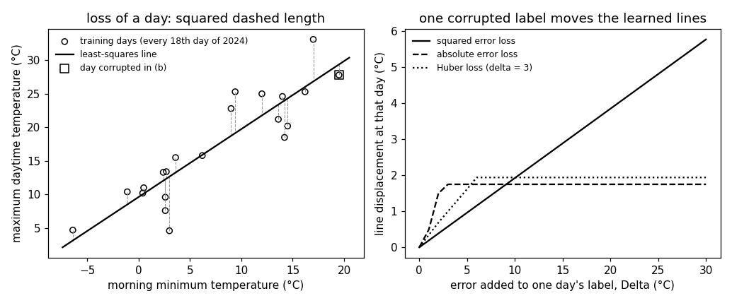
  [ok] [B-loss] least-squares line h(x) = 9.62 + 1.01 x
  [ok] [B-loss] 2024-01-01: morning minimum 2.6, maximum 9.6, prediction 12.3, squared error loss 7.05
  [ok] [B-loss] largest loss 64.95 on 2024-12-08 (morning minimum 3.0, maximum 4.6, prediction 12.66); smallest 0.01
  [ok] [B-loss] the average of the 21 losses, the training error, is 12.75, its square root 3.57 degrees
  [ok] [B-loss] normal equations: the gradient of the average loss, -(2/m) X^T (y - X w), vanishes at the least-squares line
  [ok] [B-loss] 500 other lines all have a larger average squared error loss (the average loss is convex with the least-squares line as its unique minimizer)
  [ok] [B-loss] the squared error loss is unit-free up to the square: the losses are measured in squared degrees, the labels in degrees
Constant predictions: the average squared error of a constant c is the sample variance of the labels plus (c - mean)^2, so the sample mean is the best constant; the median is the best constant under the absolute error.
print("[B-constant] constant predictions under the squared and the absolute "
      "error")
ybar, ymed = float(y.mean()), float(np.median(y))
var_y = float(np.mean((y - ybar) ** 2))
grid = np.linspace(y.min() - 5, y.max() + 5, 20001)
sq_const = np.array([np.mean((y - c) ** 2) for c in grid])
abs_const = np.array([np.mean(np.abs(y - c)) for c in grid])
check(f"[B-constant] average squared error of a constant c equals the "
      f"sample variance {var_y:.2f} plus (c - mean)^2 for every c",
      np.allclose(sq_const, var_y + (grid - ybar) ** 2))
check(f"[B-constant] the sample mean {ybar:.2f} is the best constant under "
      f"the squared error loss (average {var_y:.2f})",
      abs(grid[np.argmin(sq_const)] - ybar) < 2e-3)
check(f"[B-constant] the median {ymed:.2f} is the best constant under the "
      f"absolute error loss (average {abs_const.min():.2f})",
      abs(grid[np.argmin(abs_const)] - ymed) < 2e-3)
check(f"[B-constant] the least-squares line lowers the average squared "
      f"error from {var_y:.2f} (best constant) to {train_err:.2f}",
      train_err < var_y)
[B-constant] constant predictions under the squared and the absolute error
  [ok] [B-constant] average squared error of a constant c equals the sample variance 62.05 plus (c - mean)^2 for every c
  [ok] [B-constant] the sample mean 17.14 is the best constant under the squared error loss (average 62.05)
  [ok] [B-constant] the median 15.80 is the best constant under the absolute error loss (average 6.83)
  [ok] [B-constant] the least-squares line lowers the average squared error from 62.05 (best constant) to 12.75
Gaussian noise: the negative log-likelihood of a label is an increasing affine function of its squared error loss, so the least-squares line is the maximum likelihood estimate, and the training error is the maximum likelihood variance.
print("[B-gauss] Gaussian noise: negative log-likelihood vs squared error")


def nll(w, sigma2, x, y):
    """Negative log-likelihood of the labels under y = h(x) + Gaussian
    noise of variance sigma2."""
    return float(np.sum(sq_loss(w, x, y) / (2 * sigma2)
                        + 0.5 * np.log(2 * np.pi * sigma2)))


sigma2 = train_err
check("[B-gauss] for every line, the negative log-likelihood equals "
      "m/(2 sigma^2) times the average squared error loss plus "
      "(m/2) ln(2 pi sigma^2)",
      all(abs(nll(w, sigma2, x, y)
              - (m / (2 * sigma2) * sq_loss(w, x, y).mean()
                 + m / 2 * np.log(2 * np.pi * sigma2))) < 1e-9
          for w in others))
check("[B-gauss] the least-squares line has the smallest negative "
      "log-likelihood among the 501 lines, for every noise variance",
      all(nll(w_ls, s2, x, y) < min(nll(w, s2, x, y) for w in others)
          for s2 in (1.0, sigma2, 100.0)))
s2_grid = np.linspace(1.0, 60.0, 5901)
nll_s2 = np.array([nll(w_ls, s2, x, y) for s2 in s2_grid])
check(f"[B-gauss] the maximum likelihood noise variance is the training "
      f"error {train_err:.2f}",
      abs(s2_grid[np.argmin(nll_s2)] - train_err) < 1e-2)
[B-gauss] Gaussian noise: negative log-likelihood vs squared error
  [ok] [B-gauss] for every line, the negative log-likelihood equals m/(2 sigma^2) times the average squared error loss plus (m/2) ln(2 pi sigma^2)
  [ok] [B-gauss] the least-squares line has the smallest negative log-likelihood among the 501 lines, for every noise variance
  [ok] [B-gauss] the maximum likelihood noise variance is the training error 12.75
One training day's label is raised by Delta = 0, ..., 30 degrees; the least-squares line moves in proportion to Delta (the proportionality constant is the day's leverage), while the least-absolute-deviation line and the Huber line stop moving once the corrupted day is far from them.
print("[B-outlier] one day's label raised by Delta: least squares, least "
      "absolute deviation, Huber")


def lad(X, x, y):
    """Least absolute deviation line: an optimal line passes through two
    training days with distinct mornings (a vertex of the linear program),
    so the exact minimizer is found by enumerating the pairs."""
    best, best_val = None, np.inf
    for i in range(len(x)):
        for j in range(i + 1, len(x)):
            if x[i] == x[j]:
                continue
            w1 = (y[j] - y[i]) / (x[j] - x[i])
            w = np.array([y[i] - w1 * x[i], w1])
            val = abs_loss(w, x, y).mean()
            if val < best_val - 1e-12:
                best, best_val = w, val
    return best, best_val


def huber_loss(r, delta):
    a = np.abs(r)
    return np.where(a <= delta, r ** 2, 2 * delta * a - delta ** 2)


def huber(X, x, y, delta, iters=500):
    """Huber line by iteratively reweighted least squares: the fixed
    point of w <- argmin sum_i c_i (y_i - h(x_i))^2 with c_i = 1 for a
    residual within delta and delta/|r_i| beyond."""
    w = least_squares(X, y)
    for _ in range(iters):
        r = y - X @ w
        c = np.where(np.abs(r) <= delta, 1.0, delta / np.maximum(np.abs(r),
                                                                 1e-12))
        w_new = np.linalg.solve(X.T @ (c[:, None] * X), X.T @ (c * y))
        if np.max(np.abs(w_new - w)) < 1e-12:
            w = w_new
            break
        w = w_new
    return w


DELTA_HUBER = 3.0
r_day = int(np.argmax(x))          # the training day with the warmest morning
H = X @ np.linalg.solve(X.T @ X, X.T)
leverage = float(H[r_day, r_day])
w_lad0, _ = lad(X, x, y)
w_hub0 = huber(X, x, y, DELTA_HUBER)
check(f"[B-outlier] corrupted day {dates[r_day]}: morning minimum "
      f"{x[r_day]:.1f}, maximum {y[r_day]:.1f}; its leverage is "
      f"{leverage:.3f}", 0 < leverage < 1)
check(f"[B-outlier] clean lines: least squares {w_ls[0]:.2f} + "
      f"{w_ls[1]:.2f} x, least absolute deviation {w_lad0[0]:.2f} + "
      f"{w_lad0[1]:.2f} x, Huber (delta = {DELTA_HUBER:.0f}) "
      f"{w_hub0[0]:.2f} + {w_hub0[1]:.2f} x",
      abs(w_lad0[1] - w_ls[1]) < 0.5)
r_hub = y - X @ w_hub0
grad_hub = X.T @ np.where(np.abs(r_hub) <= DELTA_HUBER, 2 * r_hub,
                          2 * DELTA_HUBER * np.sign(r_hub))
check("[B-outlier] the Huber line is a stationary point of the average "
      "Huber loss (its gradient vanishes)", np.allclose(grad_hub, 0, atol=1e-6))
deltas = np.arange(0.0, 30.5, 1.0)
disp = {"ls": [], "lad": [], "huber": []}
for d in deltas:
    y_pert = y.copy()
    y_pert[r_day] += d
    w1 = least_squares(X, y_pert)
    w2, _ = lad(X, x, y_pert)
    w3 = huber(X, x, y_pert, DELTA_HUBER)
    for key, w, w0 in (("ls", w1, w_ls), ("lad", w2, w_lad0),
                       ("huber", w3, w_hub0)):
        disp[key].append(float(line(w, x[r_day]) - line(w0, x[r_day])))
disp = {k: np.array(v) for k, v in disp.items()}
check(f"[B-outlier] least squares: the line at that morning moves by "
      f"exactly leverage times Delta, {leverage:.3f} degrees per degree; "
      f"{disp['ls'][-1]:.2f} degrees at Delta = {deltas[-1]:.0f}",
      np.allclose(disp["ls"], leverage * deltas, atol=1e-9))
w_ls30 = least_squares(X, np.where(np.arange(m) == r_day, y + 30.0, y))
check(f"[B-outlier] at Delta = 30 the least-squares slope rises from "
      f"{w_ls[1]:.2f} to {w_ls30[1]:.2f} degrees per degree",
      w_ls30[1] > w_ls[1])
lad_stop = deltas[np.argmax(np.isclose(disp["lad"], disp["lad"][-1]))]
hub_stop = deltas[np.argmax(np.isclose(disp["huber"], disp["huber"][-1],
                                       atol=1e-6))]
check(f"[B-outlier] least absolute deviation: the line moves by at most "
      f"{np.abs(disp['lad']).max():.2f} degrees and does not change beyond "
      f"Delta = {lad_stop:.0f}",
      np.abs(disp["lad"]).max() < disp["ls"][-1] / 2)
check(f"[B-outlier] Huber: the line moves by {disp['huber'][-1]:.2f} degrees "
      f"and does not change beyond Delta = {hub_stop:.0f}",
      np.allclose(disp["huber"][deltas >= hub_stop], disp["huber"][-1],
                  atol=1e-6) and disp["huber"][-1] < disp["ls"][-1])
check("[B-outlier] the displacement of the least-squares line is the "
      "largest of the three at Delta = 30",
      disp["ls"][-1] > max(abs(disp["lad"][-1]), abs(disp["huber"][-1])))
[B-outlier] one day's label raised by Delta: least squares, least absolute deviation, Huber
  [ok] [B-outlier] corrupted day 2024-07-17: morning minimum 19.5, maximum 27.8; its leverage is 0.192
  [ok] [B-outlier] clean lines: least squares 9.62 + 1.01 x, least absolute deviation 10.54 + 0.91 x, Huber (delta = 3) 10.16 + 0.95 x
  [ok] [B-outlier] the Huber line is a stationary point of the average Huber loss (its gradient vanishes)
  [ok] [B-outlier] least squares: the line at that morning moves by exactly leverage times Delta, 0.192 degrees per degree; 5.76 degrees at Delta = 30
  [ok] [B-outlier] at Delta = 30 the least-squares slope rises from 1.01 to 1.37 degrees per degree
  [ok] [B-outlier] least absolute deviation: the line moves by at most 1.75 degrees and does not change beyond Delta = 3
  [ok] [B-outlier] Huber: the line moves by 1.93 degrees and does not change beyond Delta = 6
  [ok] [B-outlier] the displacement of the least-squares line is the largest of the three at Delta = 30
CSVs for the figure and the matplotlib preview.
print("[B-plot] training days, least-squares line, displacement curves")
with open(OUT_DIR / "sqerrloss_points.csv", "w") as fh:
    fh.write("date,tmin,tmax,pred,loss,corrupted\n")
    for i in range(m):
        fh.write(f"{dates[i]},{x[i]:.1f},{y[i]:.1f},{line(w_ls, x[i]):.4f},"
                 f"{losses[i]:.4f},{int(i == r_day)}\n")
xs = np.linspace(x.min() - 1, x.max() + 1, 2)
with open(OUT_DIR / "sqerrloss_lines.csv", "w") as fh:
    fh.write("tmin,ls\n")
    for v in xs:
        fh.write(f"{v:.3f},{line(w_ls, v):.4f}\n")
with open(OUT_DIR / "sqerrloss_outlier.csv", "w") as fh:
    fh.write("delta,ls,lad,huber\n")
    for i, d in enumerate(deltas):
        fh.write(f"{d:.0f},{disp['ls'][i]:.4f},{disp['lad'][i]:.4f},"
                 f"{disp['huber'][i]:.4f}\n")
check(f"[B-plot] all {m} training days are drawn; the displacement curve "
      f"has {len(deltas)} points", len(deltas) == 31)

fig, (ax1, ax2) = plt.subplots(1, 2, figsize=(9.4, 3.9))
for i in range(m):
    ax1.plot([x[i], x[i]], [y[i], line(w_ls, x[i])], color="0.6", lw=0.7,
             ls="--")
ax1.scatter(x, y, marker="o", facecolors="none", edgecolors="black", s=28,
            label=f"training days (every {STRIDE}th day of 2024)")
ax1.plot(xs, line(w_ls, xs), "k-", label="least-squares line")
ax1.scatter([x[r_day]], [y[r_day]], marker="s", facecolors="none",
            edgecolors="black", s=60, label="day corrupted in (b)")
ax1.set_xlabel("morning minimum temperature (°C)")
ax1.set_ylabel("maximum daytime temperature (°C)")
ax1.set_title("loss of a day: squared dashed length")
ax1.legend(frameon=False, fontsize=8)
ax2.plot(deltas, disp["ls"], "k-", label="squared error loss")
ax2.plot(deltas, disp["lad"], "k--", label="absolute error loss")
ax2.plot(deltas, disp["huber"], "k:", label=f"Huber loss (delta = "
         f"{DELTA_HUBER:.0f})")
ax2.set_xlabel("error added to one day's label, Delta (°C)")
ax2.set_ylabel("line displacement at that day (°C)")
ax2.set_title("one corrupted label moves the learned lines")
ax2.legend(frameon=False, fontsize=8)
fig.tight_layout()
fig.savefig(OUT_DIR / "sqerrloss.png", dpi=110)

n_ok = sum(ok for _, ok in report)
print(f"\n{n_ok}/{len(report)} checks pass")
if n_ok != len(report):
    raise SystemExit(1)
[B-plot] training days, least-squares line, displacement curves
  [ok] [B-plot] all 21 training days are drawn; the displacement curve has 31 points

26/26 checks pass
B-plot writes when the script runs