maxlikelihood.py, which recomputes what the entry states: the script block by block · open in ColabDictionary of Applied Machine Learning: 147 machine-learning terms, each with a definition, a figure, citations and a Python demo · All terms · Demos · Start here
Updated on 2026-11-19
Readiness 88/100
See also probability distribution empirical risk minimization training error independent and identically distributed assumption variance linear regression squared error loss logistic regression logistic loss Gaussian mixture model clustering error expectation–maximization gradient descent overfitting regularization ridge regression
Maximum likelihood chooses the model parameters of a probabilistic model under which an observed dataset has the largest probability density (or probability mass), that is, the model parameters that maximize the likelihood function. The dataset is modeled as realizations of independent and identically distributed (i.i.d.) random variables (RVs) with a common probability density function (pdf) from a family indexed by the model parameters. Taking the negative logarithm turns the product of pdfs into an average of losses, so maximum likelihood is empirical risk minimization (ERM) with the negative log-likelihood as loss function; linear regression with Gaussian noise, logistic regression, and the Gaussian mixture model (GMM) are maximum likelihood under specific probabilistic models. For a normal distribution the estimates are the sample mean and the mean squared deviation; where no closed form exists, gradient descent (GD) or the expectation–maximization (EM) algorithm computes the estimate as a fixed-point iteration. Under regularity conditions the estimate converges to the true model parameters as the dataset grows and is asymptotically normal with the variance of the Cramér–Rao bound. With a large hypothesis space the estimate overfits, and adding a penalty term to the negative log-likelihood, which is maximum a posteriori estimation, or shrinking the hypothesis space regularizes it.
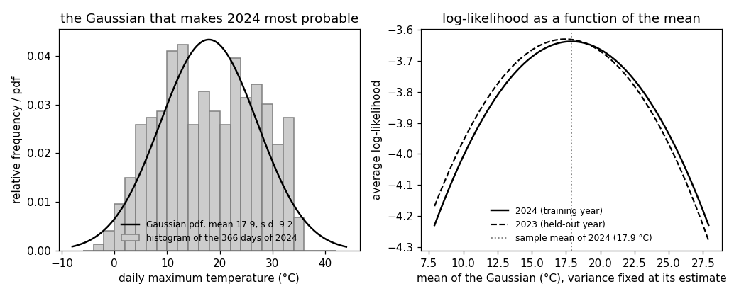
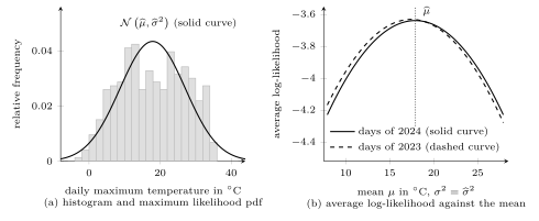
maxlikelihood.py, which recomputes what the entry states: the script block by block · open in ColabB-dataConsider the $366$ daily maximum temperatures recorded in $2024$ at the weather station Krems an der Donau. Fig. 1(a) shows their histogram. A probabilistic model for these numbers treats each of them as the realization of a random variable (RV) whose probability density function (pdf) belongs to a family indexed by a few model parameters, such as the normal distributions indexed by mean and variance. Maximum likelihood chooses the model parameters under which the recorded year is most probable: among all normal distributions, it picks the one whose pdf, evaluated at the $366$ observed temperatures and multiplied out, is largest. For the days at Krems, this is the normal distribution with mean $17.9^{\circ}$C and standard deviation $9.2^{\circ}$C, drawn in Fig. 1(a).
Formally, consider a dataset $\mathcal{D} = \{{\mathbf z}^{(1)}, \ldots, {\mathbf z}^{(m)}\}$ whose data points are realizations of independent and identically distributed (i.i.d.) RVs with a common pdf (or probability mass function (pmf)) $p^{({\mathbf z};{\mathbf w})}\left(\cdot\right)$ that depends on the model parameters ${\mathbf w} \in \mathcal{W}$. The likelihood function of ${\mathbf w}$ is the joint pdf of the dataset, viewed as a function of ${\mathbf w}$ with the dataset fixed, \begin{equation} \label{equ_maxlikelihood_likelihood_dict} L^{(\mathcal{D})}({\mathbf w}) := \prod_{r=1}^{m} p^{({\mathbf z};{\mathbf w})}\left({\mathbf z}^{(r)}\right) \text{.} \end{equation} The maximum likelihood estimate is a maximizer of the likelihood function \(\eqref{equ_maxlikelihood_likelihood_dict}\) (Casella and Berger, 2002; Fisher, 1922; Lehmann and Casella, 1998, Def. 3.1, p. 444). Since the logarithm is increasing, it is also a minimizer of the negative log-likelihood per data point, \begin{equation} \label{equ_maxlikelihood_estimate_dict} \widehat{{\mathbf w}} \in \mathop{\mathrm{arg\,min}}_{{\mathbf w} \in \mathcal{W}} \frac{1}{m} \sum_{r=1}^{m} \big( - \ln p^{({\mathbf z};{\mathbf w})}\left({\mathbf z}^{(r)}\right) \big) \text{,} \end{equation} in which the product has become a sum. The pdf is taken with respect to a base measure that does not depend on ${\mathbf w}$; changing it multiplies the likelihood function by a factor independent of ${\mathbf w}$, so the estimate is unchanged (Hastie et al., 2009, Sect. 8.2.2).
The negative log-likelihood per data point in the estimate \(\eqref{equ_maxlikelihood_estimate_dict}\) is an average loss. Each value ${\mathbf w}$ of the model parameters defines a hypothesis $h^{({\mathbf w})}$, the pdf $p^{({\mathbf z};{\mathbf w})}\left(\cdot\right)$, and the loss it incurs on a data point ${\mathbf z}$ is $L\left({\mathbf z},h^{({\mathbf w})} \right) := - \ln p^{({\mathbf z};{\mathbf w})}\left({\mathbf z}\right)$. A data point at which the pdf is small costs much, one at which it is large costs little. Maximum likelihood is therefore empirical risk minimization (ERM) over the hypothesis space $\mathcal{H} = \{h^{({\mathbf w})} : {\mathbf w} \in \mathcal{W}\}$ with the negative log-likelihood as loss function, and the minimum in the estimate \(\eqref{equ_maxlikelihood_estimate_dict}\) is the training error of the learned hypothesis $\widehat{h} = h^{(\widehat{{\mathbf w}})}$. Several machine learning (ML) methods are maximum likelihood under a specific probabilistic model. Linear regression with Gaussian noise of a fixed variance is maximum likelihood with the squared error loss (Bishop, 2006, Sect. 3.1.1). Logistic regression is maximum likelihood with the logistic loss, the negative log-likelihood of the label under a probabilistic model in which the sigmoid function of a linear function is the probability of the label (Bishop, 2006, Sect. 4.3.2). Learning a Gaussian mixture model (GMM) is maximum likelihood with the clustering error of a soft clustering, the negative logarithm of the mixture pdf (Bishop, 2006, Sect. 9.2.1).
B-closedformConsider the normal distribution $\mathcal{N}\left(\mu,\sigma^{2}\right)$ for scalar data points $x^{(1)}, \ldots, x^{(m)} \in \mathbb{R}$, so that the model parameters are ${\mathbf w} = (\mu, \sigma^{2})$. The negative log-likelihood per data point in the estimate \(\eqref{equ_maxlikelihood_estimate_dict}\) is then \begin{equation} \label{equ_maxlikelihood_gauss_dict} \frac{1}{2} \ln \big( 2 \pi \sigma^{2} \big) + \frac{1}{2 \sigma^{2} m} \sum_{r=1}^{m} \big( x^{(r)} - \mu \big)^{2} \text{.} \end{equation} For a fixed $\sigma^{2}$, the Gaussian negative log-likelihood \(\eqref{equ_maxlikelihood_gauss_dict}\) is an increasing affine function of the average squared error, so the mean with the largest likelihood function is the mean with the smallest average squared error. The zero-gradient condition for the Gaussian negative log-likelihood \(\eqref{equ_maxlikelihood_gauss_dict}\) delivers the closed form \begin{equation} \label{equ_maxlikelihood_closedform_dict} \widehat{\mu} = \frac{1}{m} \sum_{r=1}^{m} x^{(r)} \text{,} \qquad \widehat{\sigma}^{2} = \frac{1}{m} \sum_{r=1}^{m} \big( x^{(r)} - \widehat{\mu} \big)^{2} \text{,} \end{equation} the sample mean and the mean squared deviation from it (Bishop, 2006, Sect. 1.2.4, Eqs. (1.55)–(1.56)). For the days at Krems, $\widehat{\mu} = 17.9^{\circ}$C and $\widehat{\sigma}^{2} = 84.6$ squared degrees, and no pair of model parameters on a fine grid around them has a larger likelihood function. Fig. 1(b) shows the average log-likelihood as a function of $\mu$ with $\sigma^{2}$ fixed at $\widehat{\sigma}^{2}$: a downward parabola with its vertex at the sample mean. The variance estimate in the closed form \(\eqref{equ_maxlikelihood_closedform_dict}\) is biased. Its expectation is $(m - 1) \sigma^{2} / m$, so it underestimates the variance by the factor $(m - 1) / m$, which is $0.997$ for the $366$ days (Bishop, 2006, Sect. 1.2.4, Eq. (1.58)). The closed form is computed in one step, so there is no iteration to read as a fixed-point iteration.
For a GMM, for logistic regression, and for most probabilistic models with more than a few model parameters, the zero-gradient condition has no closed-form solution, and the estimate \(\eqref{equ_maxlikelihood_estimate_dict}\) is computed by an iterative method. Gradient descent (GD) on the average negative log-likelihood is a fixed-point iteration ${\mathbf w}^{(t+1)} = \mathcal{F} \big({\mathbf w}^{(t)}\big)$ for $t = 0, 1, \ldots$, whose fixed points are the points where the gradient of the negative log-likelihood vanishes. For probabilistic models with an unobserved attribute, such as the cluster index of a GMM, the expectation–maximization (EM) algorithm (Dempster et al., 1977) is the standard fixed-point iteration: one iteration never decreases the likelihood function, and its fixed points are again points with vanishing gradient (Bishop, 2006, Sect. 9.2.2). The negative log-likelihood of a GMM is not convex, so either method can stop at a local minimum (Bishop, 2006, Sect. 9.2.2).
B-loglikHow close is $\widehat{{\mathbf w}}$ to the model parameters ${\mathbf w}^{\star}$ of the probability distribution that generated the dataset? This is the generalization question for maximum likelihood, posed under the independent and identically distributed assumption (i.i.d. assumption). The expectation of the loss $L\left({\mathbf z},h^{({\mathbf w})} \right)$ under $p^{({\mathbf z};{\mathbf w}^{\star})}\left(\cdot\right)$ is the risk of $h^{({\mathbf w})}$. It exceeds the risk of $h^{({\mathbf w}^{\star})}$ by the Kullback–Leibler divergence (KL divergence) from $p^{({\mathbf z};{\mathbf w}^{\star})}\left(\cdot\right)$ to $p^{({\mathbf z};{\mathbf w})}\left(\cdot\right)$, which is nonnegative (Bishop, 2006, Sect. 1.6.1). The true model parameters therefore minimize the risk, and maximum likelihood minimizes its empirical counterpart. Consider a single model parameter $w \in \mathcal{W} \subseteq \mathbb{R}$ with a true value $w^{\star}$ in the interior of $\mathcal{W}$. Assume that the pdf is smooth in $w$, that distinct values of $w$ give distinct probability distributions, and that the support of the pdf does not depend on $w$. Then the zero-gradient condition of the log-likelihood has, with probability tending to one as $m \to \infty$, a root $\widehat{w}$ that converges in probability to $w^{\star}$ (Lehmann and Casella, 1998, Thm. 3.7, p. 447). Maximum likelihood is consistent. Any such consistent sequence of roots is asymptotically normal: with the Fisher information $I(w) := \mathbb{E} \big\{ \big( \frac{\partial}{\partial w} \ln p^{({\mathbf z};w)}\left({\mathbf z}\right) \big)^{2} \big\}$ of one data point, \begin{equation} \label{equ_maxlikelihood_normal_dict} \sqrt{m} \big( \widehat{w} - w^{\star} \big) \to \mathcal{N}\left(0,1 / I(w^{\star})\right) \quad \text{in distribution as } m \to \infty \text{,} \end{equation} (Hastie et al., 2009, Sect. 8.2.2, Eq. (8.16); Lehmann and Casella, 1998, Thm. 3.10, p. 449). The information inequality, also known as the Cramér–Rao bound, states that no unbiased estimator of $w$ that is computed from $m$ data points and satisfies mild regularity conditions has a variance below $1 / (m I(w))$ (Cramér, 1946; Lehmann and Casella, 1998, Thm. 5.10, p. 120). The asymptotic normality \(\eqref{equ_maxlikelihood_normal_dict}\) says that the variance of $\widehat{w}$ approaches this bound, which is why maximum likelihood is called asymptotically efficient. For the mean of a normal distribution with known variance $\sigma^{2}$, the Fisher information is $I(\mu) = 1 / \sigma^{2}$, and the sample mean attains the bound exactly: its variance is $\sigma^{2} / m$. For the days at Krems, the standard deviation of $\widehat{\mu}$ is therefore $\widehat{\sigma} / \sqrt{366} = 0.48^{\circ}$C. The second derivative of the parabola in Fig. 1(b) is $-1 / \widehat{\sigma}^{2}$, the Fisher information with a minus sign. The $365$ days of $2023$ give a second parabola in the same panel, with its vertex at the $2023$ mean of $17.4^{\circ}$C, half a degree from the $2024$ estimate.
B-hypospaceMaximum likelihood chooses the model parameters that are best
for the training set, and with a large hypothesis space this is
overfitting (Murphy, 2012, Sect. 7.5.1). Enlarging the
hypothesis space for the days at Krems shows the effect. With
twelve means, one per calendar month, and one common
variance, the average log-likelihood rises from $-3.64$ to
$-2.84$ on the $366$ days of $2024$. It also rises, from $-3.63$
to $-3.12$, on the $365$ days of $2023$, which did not enter the
estimate: the seasons are real, so the larger hypothesis space
helps on new data too. With one mean per calendar day,
maximum likelihood places every mean on its observation,
and the variance estimate is zero. The likelihood function
of $2024$ then exceeds every bound as $\sigma \to 0$, while the
average log-likelihood of $2023$ under the same
model parameters falls below every bound: $-22$ at $\sigma =
1^{\circ}$C and $-2083$ at $\sigma = 0.1^{\circ}$C. The same
singularity is present in a
GMM with a component whose mean coincides with one
data point and whose variance shrinks to zero
(Bishop, 2006, Sect. 9.2.1). Both remedies are forms of
regularization. One shrinks the hypothesis space: fewer
means, or a lower bound on the variance. The other
adds a penalty term to the negative log-likelihood. This
is maximum a posteriori (MAP) estimation,
\begin{equation}
\label{equ_maxlikelihood_map_dict}
\widehat{{\mathbf w}} \in \mathop{\mathrm{arg\,min}}_{{\mathbf w} \in \mathcal{W}}
\frac{1}{m} \sum_{r=1}^{m}
\big( - \ln p^{({\mathbf z};{\mathbf w})}\left({\mathbf z}^{(r)}\right)
\big) - \frac{1}{m} \ln p^{({\mathbf w})}\left({\mathbf w}\right)
\text{,}
\end{equation}
in which the penalty term is the negative logarithm of a
prior distribution with pdf $p^{({\mathbf w})}\left(\cdot\right)$ over the
model parameters. A minimizer of the penalized negative
log-likelihood \(\eqref{equ_maxlikelihood_map_dict}\) maximizes the
posterior distribution of ${\mathbf w}$ given the dataset
(Bishop, 2006, Sect. 1.2.5, Eq. (1.67)). A Gaussian
prior distribution on the weight vector of linear regression
gives ridge regression (Murphy, 2012, Sect. 7.5.1). A
Gaussian prior distribution $\mathcal{N}\left(\mu_{0},\tau^{2}\right)$ on the
mean of a normal distribution with known $\sigma^{2}$ moves
the estimate from the sample mean $\widehat{\mu}$ toward
$\mu_{0}$, to $(m \tau^{2} \widehat{\mu} + \sigma^{2}
\mu_{0}) / (m \tau^{2} + \sigma^{2})$
(Bishop, 2006, Sect. 2.3.6, Eq. (2.141)). The
penalty term in the MAP estimate
\(\eqref{equ_maxlikelihood_map_dict}\) is divided by $m$,
so it vanishes as the dataset grows, and the MAP estimate
approaches the maximum likelihood estimate.
pythondemos/maxlikelihood.py
See also: likelihood function, probabilistic model, probability distribution, probability density function, model parameter, estimator, empirical risk minimization, loss function, training error, risk, independent and identically distributed assumption, normal distribution, sample mean, variance, linear regression, squared error loss, logistic regression, logistic loss, Gaussian mixture model, clustering error, expectation–maximization, gradient descent, fixed-point iteration, zero-gradient condition, Kullback–Leibler divergence, overfitting, regularization, penalty term, prior distribution, posterior distribution, ridge regression, optimization problem.
@misc{dictml_maxlikelihood,
  author = {Jung, Alexander},
  editor = {Olioumtsevits, Konstantina and Schnoor, Ekkehard},
  title = {maximum likelihood},
  howpublished = {Dictionary of Applied Machine Learning (course edition)},
  year = {2026},
  doi = {10.5281/zenodo.21569296},
  note = {ISBN 978-952-64-3013-3, CC BY 4.0, retrieved 2026-11-20},
  url = {https://dictionaryofml.org/terms/maxlikelihood.html}
}