independent and identically distributed (i.i.d.)

Jung, Alexander

independent and identically distributed (i.i.d.)

Updated on 2026-09-22

Typeset PDF version — the authoritative form of this entry

Python demo — a script that recomputes what this entry states and prints one line per check

A collection of random variables (RVs) is independent and identically distributed (i.i.d.) if every member follows the same probability distribution and the members are jointly independent. Joint independence is a product rule: the probability of any combination of their values is the product of one probability per RV. Independence is a statement about the RVs jointly, so it presupposes that they are defined on one common probability space. A widely used probabilistic model for the generation of data points is a collection of i.i.d. RVs. This i.i.d. assumption defines the risk of a hypothesis and makes the average loss on a training set an unbiased estimate of it. Whether a given dataset can be represented this way is checked by comparing the empirical distributions of its blocks and by testing the data points for dependence.

Definition

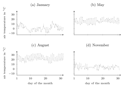
B-monthsA weather station at Krems an der Donau measured the air temperature every ten minutes throughout 2024. Fig. 1 shows four of those months, each a dataset of more than $4000$ numbers. A convenient reading of one such month takes its numbers as interchangeable draws from one source, so that only how often each value occurs matters and not which measurement is read. That reading is the i.i.d. probabilistic model, and the figure shows two facts it does not represent. The four months have different averages, $1.35$ degrees in January against $22.97$ in August, so a probability distribution fitted to one month does not describe another. Inside every month the temperature rises and falls once a day, so a measurement almost repeats the one ten minutes earlier, with a correlation above $0.99$ in each of the four months.

Figure 1 of the entry iid — Figure 1: Air temperature at Krems, measured every ten minutes, for four months of 2024 (timestamps in UTC). Each month is read as one dataset. The averages differ from month to month, and the temperature rises and falls once a day within each month. Data generated by `pythondemos/iid.py`

A collection of random variables (RVs) $\datapoint^{(1)}, \ldots, \datapoint^{(\samplesize)}$, all defined on one common probability space $\probspace$ and taking values in a measurable space $\datapointspace$, is i.i.d. if every $\datapoint^{(\sampleidx)}$ follows the same probability distribution and the RVs are mutually independent. Independence is a product rule: for any measurable sets $\genericevent_{1}, \ldots, \genericevent_{\samplesize} \subseteq \datapointspace$, \begin{equation} \label{eq:iid_product} \prob{ \datapoint^{(1)} \in \genericevent_{1}, \ldots, \datapoint^{(\samplesize)} \in \genericevent_{\samplesize}} = \prod_{\sampleidx=1}^{\samplesize} \prob{ \datapoint^{(\sampleidx)} \in \genericevent_{\sampleidx}} \text{.} \end{equation} The common probability space is what makes the left-hand side of the product rule $\eqref{eq:iid_product}$ well defined: one outcome has to fix all $\samplesize$ values at once, so a separate probability space per RV leaves the joint probability undefined (see RV). Such a common space always exists: probability theory constructs independent copies of a given RV on one probability space (Klenke, 2020, Th. 2.19).

B-shuffleThe two requirements are separate, and the Krems record violates each of them for a different reason. Taking the maximum of each day leaves $366$ numbers for the year and removes the daily cycle of Fig. 1, so the two requirements can be examined one at a time. January averages $5.95$ degrees and July $28.99$, so which day is read decides the probability distribution of the value. Subtracting the seasonal average removes this first violation: the twelve monthly averages of what is left agree to within $0.55$ degrees. The second violation remains, since consecutive values of the remainder still have a Pearson correlation coefficient of $0.67$. 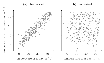Permuting the record at random separates the two in the other direction. A permutation leaves every recorded value and its frequency exactly as it was, and it destroys the dependence: a day above $25$ degrees is followed by another such day $3.3$ times as often as the product rule $\eqref{eq:iid_product}$ allows, whereas after permuting, two such days in a row occur with frequency $0.071$ against the $0.070$ that the product rule predicts, and the Pearson correlation coefficient of consecutive values falls from $0.94$ to $0.035$ (see Fig. 2). The remaining combination occurs as well: two sensors of different accuracy, read once each, deliver independent values that are not identically distributed.

Figure 2 of the entry iid — Figure 2: Each of the $365$ pairs of consecutive days at Krems in 2024, plotted by the maximum temperature of the first day against that of the second. (a) In the order measured, a warm day follows a warm day. (b) After a random permutation of the same $366$ numbers, which changes no value and no frequency, nothing relates the two coordinates. Independence is a property of the joint probability distribution, not of the values a single RV takes. Data generated by `pythondemos/iid.py`

One probability distribution then describes the entire collection: the product rule $\eqref{eq:iid_product}$ writes every joint probability in terms of $\samplesize$ copies of a single probability distribution, so a collection of any size is described by as many numbers as one RV is. Averages over the collection then estimate features of that one probability distribution. Let $\sigma^{2}$ be the common variance of real-valued i.i.d. RVs. Their sample mean $(1/\samplesize) \sum_{\sampleidx=1}^{\samplesize} \datapoint^{(\sampleidx)}$ then has the common expectation as its own expectation and variance $\sigma^{2}/\samplesize$, so it concentrates around that expectation as the collection grows. For $\sigma^{2} \leq 1$, Chebyshev's inequality turns this into a bound: the sample mean is within $\sqrt{1/(\delta \samplesize)}$ of the common expectation with probability at least $1-\delta$, for every $\delta \in (0,1)$ (Shalev-Shwartz and Ben-David, 2014, Lemma B.2). The law of large numbers and the concentration inequalities state how fast: for RVs confined to an interval $[a,b]$, Hoeffding's inequality bounds the probability that the sample mean deviates from the common expectation by more than $\epsilon$ by $2 \exp \big( -2 \samplesize \epsilon^{2}/(b-a)^{2} \big)$ (Hoeffding, 1963; Shalev-Shwartz and Ben-David, 2014, Lemma B.6). Both halves of the property are needed: dependence adds covariance terms to the variance of the sample mean, and RVs with different probability distributions have no common expectation for the sample mean to concentrate around.

The analysis of machine learning (ML) methods is often based on approximating the generation of data points as i.i.d. RVs with one unknown probability distribution (Shalev-Shwartz and Ben-David, 2014, Sect. 2.3.1). This probabilistic model is the i.i.d. assumption. It defines the risk of a hypothesis as the expected loss $\expect \big\{ \lossfunc{\datapoint}{\hypothesis} \big\}$ on a data point drawn from that probability distribution, and it makes the average loss on a training set an unbiased estimate of the risk (Shalev-Shwartz and Ben-David, 2014, Sect. 4.2). This is the argument for empirical risk minimization (ERM) and for using a validation set to estimate the loss outside the training set (Shalev-Shwartz and Ben-David, 2014, Th. 11.1). A distribution shift violates the identically distributed requirement across datasets: the probability distribution that generated the training set differs from the one that generates the data points encountered after deployment.

There are established statistical methods to verify whether a given dataset can be approximated by realizations of i.i.d. RVs, one for each requirement. To verify that the data points are realizations of RVs with a common probability distribution, cut the dataset into blocks of equal size and compare two blocks by the largest vertical gap between their empirical cumulative distribution functions (cdfs). That gap is the two-sample Kolmogorov–Smirnov statistic (Gretton et al., 2012, Sect. 7.2.1). It is at most one, and it equals one when the two blocks share no value. To verify that the data points are realizations of independent RVs, compare the Pearson correlation coefficient between values a fixed number of positions apart against the same correlation computed after reordering the values at random. If the RVs were i.i.d., every ordering of the observed values would be equally likely, so no ordering is special and the observed correlation should be an unremarkable member of that collection of reordered ones. This comparison is a permutation test, a form of hypothesis testing.

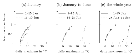
B-verifyFig. 3 applies both methods to the maximum temperature during each day, over periods of growing length. Within January the largest gap between the two $15$-day blocks is $0.33$; over January to June and over the whole year it is $1$, so two blocks of those periods share no value. These data points are therefore unlikely to be realizations of RVs with a common probability distribution. The independence check fails at every length: the Pearson correlation coefficient between the temperatures of consecutive days is $0.63$ within January, $0.91$ over January to June and $0.94$ over the year, and no reordering among $2000$ random ones reaches those values. Each method examines one requirement only: the block comparison does not detect dependence, which is why January passes it, and the permutation test does not detect a changing probability distribution, since reordering cannot change which values were recorded.

Figure 3 of the entry iid — Figure 3: Empirical cdfs of the two $15$-day blocks that are furthest apart, for three periods of the Krems record. The largest vertical gap between the two staircases is $0.33$ in (a), and $1$ in (b) and (c), where the two blocks share no value. Data generated by `pythondemos/iid.py`

A threshold settles how large a gap counts as evidence. For two blocks of $n$ values each, i.i.d. RVs produce a gap above $\sqrt{-\log(\alpha/2)/2} \cdot \sqrt{2/n}$ with probability at most $\alpha$. For $n = 15$ and $\alpha = 0.05$ that threshold is $0.50$, which the January gap of $0.33$ does not reach. The gap reported above is however the largest over every pair of blocks, $66$ pairs for January to June and $276$ for the year, so the threshold has to account for that many comparisons: dividing $\alpha$ among the pairs raises it to $0.73$ and $0.79$, and both periods still exceed it. A gap below its threshold proves nothing beyond itself: the blocks then carry no evidence against a common probability distribution, while a dependence between consecutive values can still be present. This is why both methods are used.

Which statistic to use then depends on which departure the check should detect, and that choice can be justified only once the departure is named. Optimality of a test presupposes a named alternative. Against a fixed dependent probability distribution $q$ of the whole collection, the Neyman–Pearson lemma makes the ratio of the two likelihood functions, \begin{equation} \label{eq:iid_lratio} \Lambda = \frac{q(\datapoint^{(1)}, \ldots, \datapoint^{(\samplesize)})} {\prod_{\sampleidx=1}^{\samplesize} p(\datapoint^{(\sampleidx)})} \text{,} \end{equation} the most powerful statistic at every level, and its power is determined by the Kullback–Leibler divergence (KL divergence) between $q$ and the i.i.d. probability distribution in the denominator of the ratio $\eqref{eq:iid_lratio}$. The Pearson correlation coefficient used above is a score statistic of that ratio: its logarithm, differentiated with respect to a parameter whose value zero is the i.i.d. case. Differentiating the logarithm of the Gaussian first-order autoregressive likelihood function with respect to its correlation at zero leaves exactly the Pearson correlation coefficient between consecutive values. Such a statistic is optimal against the alternatives that its parameter indexes, and against those only.

Against the unrestricted alternative no test is uniformly most powerful: dependent probability distributions come arbitrarily close to i.i.d. ones, so for every test of level $\alpha$ and every $\epsilon > 0$ there is a dependent probability distribution against which its power stays below $\alpha + \epsilon$. Two weaker optimality statements still hold. A permutation test keeps its level exactly, whatever statistic it uses, for the composite null hypothesis of i.i.d. RVs with an unknown common probability distribution. The argument is one line. Under that hypothesis the joint probability distribution of $\datapoint^{(1)}, \ldots, \datapoint^{(\samplesize)}$ is the same product $\eqref{eq:iid_product}$ for every ordering of the values, so all $\samplesize!$ orderings are equally likely. The observed ordering is therefore one draw from the $\samplesize!$ reorderings, and the statistic computed on random reorderings has exactly the probability distribution of the observed statistic. The second statement takes the opposite route: on a finite set of values a statistic built from observed frequencies alone, with no alternative named at all, still attains the best achievable error exponent (Cover and Thomas, 2006).

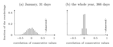
B-optimalFig. 4 shows the reordered correlations for two datasets: the maximum temperatures of the $31$ days of January, and of the $366$ days of the whole year. They are centered at zero, with a spread of $0.177$ for January and $0.052$ for the year. Both agree with $1/\sqrt{\samplesize}$ ($0.180$ and $0.052$), the standard deviation of a Pearson correlation coefficient computed from $\samplesize$ independent values. The observed $0.63$ and $0.94$ exceed every one of the $2000$ reordered values, and the longer dataset separates them more sharply, since the reordered values crowd more tightly around zero as $\samplesize$ grows.

Figure 4 of the entry iid — Figure 4: The Pearson correlation coefficient between consecutive values for $2000$ random reorderings of the same numbers, against the value the record itself gives. Because all orderings are equally likely for i.i.d. RVs, the reordered values are what the Pearson correlation coefficient would look like if the representation held. They are centered at zero and their spread narrows from $0.177$ on $31$ days to $0.052$ on $366$, so the same statistic separates more sharply on the longer dataset. Data generated by `pythondemos/iid.py`

See also: RV, probability distribution, probability space, event, data point, realization, risk, law of large numbers, empirical distribution, hypothesis testing, distribution shift.

References

Klenke (2020). Probability Theory: A Comprehensive Course. Springer Nature. doi.org/10.1007/978-3-030-56402-5
Shalev-Shwartz and Ben-David (2014). Understanding Machine Learning: From Theory to Algorithms. Cambridge Univ. Press. doi.org/10.1017/cbo9781107298019
Hoeffding (1963). Probability Inequalities for Sums of Bounded Random Variables. J. Amer. Statistical Assoc.. doi.org/10.1080/01621459.1963.10500830
Gretton et al. (2012). A Kernel Two-Sample Test. Journal of Machine Learning Research. www.jmlr.org/papers/v13/gretton12a.html
Cover and Thomas (2006). Elements of Information Theory. Wiley. doi.org/10.1002/047174882X

Cite this entry

@misc{dictml_iid,
  author = {Jung, Alexander},
  editor = {Olioumtsevits, Konstantina and Schnoor, Ekkehard},
  title = {independent and identically distributed (i.i.d.)},
  howpublished = {Dictionary of Applied Machine Learning (course edition)},
  year = {2026},
  doi = {10.5281/zenodo.21569296},
  note = {ISBN 978-952-64-3013-3, CC BY 4.0, retrieved 2026-09-23},
  url = {https://dictionaryofml.org/terms/iid.html}
}