B-plot writes when the script runsDictionary of Applied Machine Learning · independent and identically distributed (i.i.d.)
Numerical companion to the entry independent and identically distributed (i.i.d.): it recomputes what the entry states and prints one line per check
The entry asks whether temperature measurements recorded at Krems in 2024 can be modeled as i.i.d. random variables, and answers it by testing the two halves of the definition separately on the record itself. Self-contained (numpy/matplotlib only), fixed seed; the measurements are fetched from the public GeoSphere Austria archive.
Run it with python3 iid.py, from any directory — it writes its output files into the current directory. Requires NumPy and Matplotlib only, and uses fixed seeds, so the printed numbers reproduce exactly. Download iid.py · Notebook · Open in Colab
One cell per block of the script: the code, and what that code printed when it last ran here
"""
iid.py — numerical companion to the glossary entry 'independent and
identically distributed (i.i.d.)'.

The entry asks whether temperature measurements recorded at Krems in 2024 can
be modeled as i.i.d. random variables, and answers it by testing the two halves
of the definition separately on the record itself. Self-contained
(numpy/matplotlib only), fixed seed; the measurements are fetched from the
public GeoSphere Austria archive.

Blocks
------
[B-months]      Air temperature every ten minutes for January, May, August and
                November, one dataset per month. The levels differ across the
                months and the daily cycle repeats inside each of them, which
                is what the rest of the entry measures.
[B-data]        366 daily maximum temperatures at Krems an der Donau
                (station 3805) for 2024.
[B-identical]   The identically distributed half fails: the monthly averages
                run from January to July, so the distribution of the
                temperature depends on which day is read.
[B-independent] The independent half fails too: the event "above 25 degrees"
                has probability 0.265 per day, so under independence two
                consecutive days would both exceed it with probability 0.070;
                the record does it three times as often. The lag-one
                correlation says the same.
[B-shuffle]     A random permutation of the same 366 numbers leaves the
                collection of values untouched and makes the product rule
                hold, which is what independence is about. Writes the two
                panels of the entry's second figure.
[B-deseason]    Subtracting the seasonal average repairs the identically
                distributed half only: the lag-one correlation of what is
                left is still 0.67.
[B-verify]      The two standard methods applied to periods of growing length
                (January, January to June, the whole year): the largest gap
                between the empirical CDFs of two 15-day blocks of the period
                against the Kolmogorov-Smirnov threshold, and the lag-one
                correlation calibrated by a permutation test. Writes the
                panels of the entry's third figure.
[B-optimal]     The same statistic on one month and on one year: the
                correlation of consecutive values over random reorderings,
                which tightens
                as the collection grows. Writes the panels of the entry's
                last figure.

Outputs
-------
iid_temps.csv            : date, daily maximum temperature, 366 days of 2024
iid_month_<mon>.csv      : day, temperature every ten minutes, four months
iid_lag_record.csv       : today, tomorrow -- the record, for the left panel
iid_lag_shuffled.csv     : today, tomorrow -- one permutation, right panel
iid_cdf_<period>_<block>.csv : temperature, fraction -- empirical CDFs
iid_perm_<period>.csv    : center, fraction -- the correlation of consecutive
                           values over random reorderings
iid.png                  : preview (checking only)

Data generated by pythondemos/iid.py.
"""

import json
import math
import urllib.request
from pathlib import Path

import numpy as np
import matplotlib

matplotlib.use("Agg")
import matplotlib.pyplot as plt

OUT_DIR = Path(__file__).parent
ARCHIVE = "https://dataset.api.hub.geosphere.at/v1/station/historical/"
STATION = 3805

report = []


def check(name, ok):
    report.append((name, bool(ok)))
    print(f"  [{'ok' if ok else 'FAIL'}] {name}")


def fetch(resource, parameter, start, end):
    """One parameter of one station from the GeoSphere Austria archive."""
    url = (f"{ARCHIVE}{resource}?parameters={parameter}"
           f"&station_ids={STATION}&start={start}&end={end}")
    with urllib.request.urlopen(url, timeout=180) as resp:
        payload = json.load(resp)
    values = payload["features"][0]["properties"]["parameters"]
    key = list(values.keys())[0]
    return (np.array(values[key]["data"], dtype=float),
            [t[:16] for t in payload["timestamps"]])


def lag_one_correlation(x):
    """Pearson correlation coefficient between consecutive entries of x."""
    return float(np.corrcoef(x[:-1], x[1:])[0, 1])


def ks_statistic(a, b):
    """Largest gap between the empirical CDFs of two collections."""
    grid = np.sort(np.concatenate([a, b]))
    fa = np.searchsorted(np.sort(a), grid, side="right") / len(a)
    fb = np.searchsorted(np.sort(b), grid, side="right") / len(b)
    return float(np.abs(fa - fb).max())


def ks_threshold(size, level):
    """Two-sample Kolmogorov-Smirnov critical value for two blocks of size."""
    return math.sqrt(-0.5 * math.log(level / 2)) * math.sqrt(2 / size)


def empirical_cdf(x):
    """Sorted values and the fraction of the collection at or below each."""
    values = np.sort(x)
    return values, np.arange(1, len(values) + 1) / len(values)
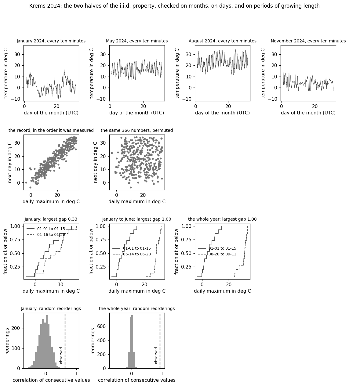
Air temperature every ten minutes for January, May, August and November, one dataset per month. The levels differ across the months and the daily cycle repeats inside each of them, which is what the rest of the entry measures.
MONTHS = [(1, "jan", "January"), (5, "may", "May"),
          (8, "aug", "August"), (11, "nov", "November")]
fine = {}
for number, tag, title in MONTHS:
    last = 31 if number in (1, 8) else 30
    values, stamps = fetch("klima-v2-10min", "TL",
                           f"2024-{number:02d}-01T00:00",
                           f"2024-{number:02d}-{last:02d}T23:50")
    day = np.array([int(s[8:10]) + int(s[11:13]) / 24 + int(s[14:16]) / 1440
                    for s in stamps])
    fine[tag] = (day, values, title)
    with open(OUT_DIR / f"iid_month_{tag}.csv", "w") as f:
        f.write("day,temp\n")
        for a, b in zip(day, values):
            f.write(f"{a:.4f},{b:g}\n")
    print(f"[B-months] {title}: {len(values)} measurements, mean "
          f"{values.mean():.2f} deg, lag-one correlation "
          f"{lag_one_correlation(values):.3f}")
check("[B-months] every month is measured every ten minutes",
      all(len(fine[tag][1]) in (4320, 4464) for _, tag, _ in MONTHS))
check("[B-months] the monthly levels differ by more than twenty degrees",
      fine["aug"][1].mean() - fine["jan"][1].mean() > 20.0)
check("[B-months] consecutive measurements are nearly equal in every month",
      all(lag_one_correlation(fine[tag][1]) > 0.98 for _, tag, _ in MONTHS))
[B-months] January: 4464 measurements, mean 1.35 deg, lag-one correlation 0.997
[B-months] May: 4320 measurements, mean 16.46 deg, lag-one correlation 0.996
[B-months] August: 4464 measurements, mean 22.97 deg, lag-one correlation 0.996
[B-months] November: 4320 measurements, mean 4.19 deg, lag-one correlation 0.996
  [ok] [B-months] every month is measured every ten minutes
  [ok] [B-months] the monthly levels differ by more than twenty degrees
  [ok] [B-months] consecutive measurements are nearly equal in every month
366 daily maximum temperatures at Krems an der Donau (station 3805) for 2024.
temp, stamps = fetch("klima-v2-1d", "tlmax", "2024-01-01", "2024-12-31")
month = np.array([int(s[5:7]) for s in stamps])
with open(OUT_DIR / "iid_temps.csv", "w") as f:
    f.write("date,tlmax\n")
    for day, value in zip(stamps, temp):
        f.write(f"{day[:10]},{value:g}\n")
print(f"[B-data] {len(temp)} daily maxima, mean {temp.mean():.2f} deg, "
      f"variance {temp.var(ddof=1):.2f} deg squared")
check("[B-data] the year has all 366 days", len(temp) == 366)
check("[B-data] the record matches the archive (Feb 1: 10.4 deg)",
      stamps[31][:10] == "2024-02-01" and np.isclose(temp[31], 10.4))
[B-data] 366 daily maxima, mean 17.91 deg, variance 84.87 deg squared
  [ok] [B-data] the year has all 366 days
  [ok] [B-data] the record matches the archive (Feb 1: 10.4 deg)
The identically distributed half fails: the monthly averages run from January to July, so the distribution of the temperature depends on which day is read.
jan, jul = temp[month == 1], temp[month == 7]
print(f"[B-identical] January averages {jan.mean():.2f} deg and July "
      f"{jul.mean():.2f} deg")
check("[B-identical] the July average exceeds the January average by more "
      "than twenty degrees", jul.mean() - jan.mean() > 20.0)
check("[B-identical] the gap is large against the spread within a month",
      jul.mean() - jan.mean() > 4.0 * max(jan.std(ddof=1), jul.std(ddof=1)))
[B-identical] January averages 5.95 deg and July 28.99 deg
  [ok] [B-identical] the July average exceeds the January average by more than twenty degrees
  [ok] [B-identical] the gap is large against the spread within a month
The independent half fails too: the event "above 25 degrees" has probability 0.265 per day, so under independence two consecutive days would both exceed it with probability 0.070; the record does it three times as often. The lag-one correlation says the same.
THRESHOLD = 25.0
warm = temp > THRESHOLD
p_single = warm.mean()
p_pair = (warm[:-1] & warm[1:]).mean()
print(f"[B-independent] a day above {THRESHOLD:g} deg has frequency "
      f"{p_single:.3f}; two in a row {p_pair:.3f} against the product "
      f"{p_single ** 2:.3f}, a factor of {p_pair / p_single ** 2:.2f}")
print(f"[B-independent] lag-one correlation of the record "
      f"{lag_one_correlation(temp):.3f}")
check("[B-independent] consecutive warm days are at least three times as "
      "frequent as the product rule allows", p_pair > 3.0 * p_single ** 2)
check("[B-independent] the lag-one correlation is above 0.9",
      lag_one_correlation(temp) > 0.9)
[B-independent] a day above 25 deg has frequency 0.265; two in a row 0.230 against the product 0.070, a factor of 3.28
[B-independent] lag-one correlation of the record 0.940
  [ok] [B-independent] consecutive warm days are at least three times as frequent as the product rule allows
  [ok] [B-independent] the lag-one correlation is above 0.9
A random permutation of the same 366 numbers leaves the collection of values untouched and makes the product rule hold, which is what independence is about. Writes the two panels of the entry's second figure.
rng = np.random.default_rng(0)
shuffled = rng.permutation(temp)
warm_s = shuffled > THRESHOLD
p_pair_s = (warm_s[:-1] & warm_s[1:]).mean()
print(f"[B-shuffle] after permuting: two warm days in a row {p_pair_s:.3f} "
      f"against the product {p_single ** 2:.3f}; lag-one correlation "
      f"{lag_one_correlation(shuffled):.3f}")
check("[B-shuffle] permuting leaves the collection of values unchanged",
      np.allclose(np.sort(shuffled), np.sort(temp)))
check("[B-shuffle] the product rule now holds to within a tenth",
      abs(p_pair_s - p_single ** 2) < 0.1 * p_single ** 2)
check("[B-shuffle] the lag-one correlation is close to zero",
      abs(lag_one_correlation(shuffled)) < 0.1)
for name, series in (("iid_lag_record.csv", temp),
                     ("iid_lag_shuffled.csv", shuffled)):
    with open(OUT_DIR / name, "w") as f:
        f.write("today,tomorrow\n")
        for a, b in zip(series[:-1], series[1:]):
            f.write(f"{a:.1f},{b:.1f}\n")
[B-shuffle] after permuting: two warm days in a row 0.071 against the product 0.070; lag-one correlation 0.035
  [ok] [B-shuffle] permuting leaves the collection of values unchanged
  [ok] [B-shuffle] the product rule now holds to within a tenth
  [ok] [B-shuffle] the lag-one correlation is close to zero
Subtracting the seasonal average repairs the identically distributed half only: the lag-one correlation of what is left is still 0.67.
WINDOW = 31
wrapped = np.concatenate([temp[-(WINDOW // 2):], temp, temp[:WINDOW // 2]])
seasonal = np.convolve(wrapped, np.ones(WINDOW) / WINDOW, mode="valid")
residual = temp - seasonal
print(f"[B-deseason] after subtracting the seasonal average the monthly "
      f"means agree to {np.abs([residual[month == k].mean() for k in range(1, 13)]).max():.2f} deg, "
      f"and the lag-one correlation is still "
      f"{lag_one_correlation(residual):.3f}")
check("[B-deseason] the seasonal average is what separates January from July",
      abs(residual[month == 7].mean() - residual[month == 1].mean()) < 2.0)
check("[B-deseason] the dependence survives it",
      lag_one_correlation(residual) > 0.5)
[B-deseason] after subtracting the seasonal average the monthly means agree to 0.55 deg, and the lag-one correlation is still 0.671
  [ok] [B-deseason] the seasonal average is what separates January from July
  [ok] [B-deseason] the dependence survives it
The two standard methods applied to periods of growing length (January, January to June, the whole year): the largest gap between the empirical CDFs of two 15-day blocks of the period against the Kolmogorov-Smirnov threshold, and the lag-one correlation calibrated by a permutation test. Writes the panels of the entry's third figure.
BLOCK = 15
LEVEL = 0.05
NR_PERM = 2000
PERIODS = [("month", "January", temp[month == 1], np.array(stamps)[month == 1]),
           ("halfyear", "January to June", temp[month <= 6],
            np.array(stamps)[month <= 6]),
           ("year", "the whole year", temp, np.array(stamps))]
verdict = {}
for tag, title, series, days in PERIODS:
    nr_block = len(series) // BLOCK
    blocks = [series[i * BLOCK:(i + 1) * BLOCK] for i in range(nr_block)]
    spans = [f"{days[i * BLOCK][5:10]} to {days[(i + 1) * BLOCK - 1][5:10]}"
             for i in range(nr_block)]
    # the pair of blocks that are furthest apart, ties broken by the means
    gap, spread, first, second = max(
        (ks_statistic(blocks[i], blocks[j]),
         abs(blocks[i].mean() - blocks[j].mean()), i, j)
        for i in range(nr_block) for j in range(i + 1, nr_block))
    corr = lag_one_correlation(series)
    draws = np.array([abs(lag_one_correlation(rng.permutation(series)))
                      for _ in range(NR_PERM)])
    pvalue = (1 + (draws >= abs(corr)).sum()) / (NR_PERM + 1)
    nr_pair = nr_block * (nr_block - 1) // 2
    plain = ks_threshold(BLOCK, LEVEL)
    adjusted = ks_threshold(BLOCK, LEVEL / nr_pair)
    verdict[tag] = (title, len(series), nr_block, gap, corr, pvalue,
                    (blocks[first], spans[first]),
                    (blocks[second], spans[second]),
                    nr_pair, plain, adjusted)
    for label, index in (("early", first), ("late", second)):
        values, fraction = empirical_cdf(blocks[index])
        with open(OUT_DIR / f"iid_cdf_{tag}_{label}.csv", "w") as f:
            f.write("temp,frac\n")
            for a, b in zip(values, fraction):
                f.write(f"{a:g},{b:.4f}\n")
    print(f"[B-verify] {title} ({len(series)} days, {nr_block} blocks of "
          f"{BLOCK} days): largest gap between the empirical CDFs of two "
          f"blocks {gap:.3f} ({spans[first]} against {spans[second]}); the "
          f"correlation of consecutive values is {corr:.3f}, which no "
          f"reordering among {NR_PERM} random ones reaches")
    print(f"[B-verify] {title}: the Kolmogorov-Smirnov threshold at level "
          f"{LEVEL} is {plain:.3f} for a single pair and {adjusted:.3f} after "
          f"dividing the level among the {nr_pair} pairs; the gap "
          f"{'exceeds' if gap > adjusted else 'stays below'} it")
check("[B-verify] the gap between two blocks grows with the length of the "
      "period", verdict["month"][3] < verdict["halfyear"][3] <= verdict["year"][3])
check("[B-verify] six months and a year separate two blocks completely",
      verdict["halfyear"][3] == 1.0 and verdict["year"][3] == 1.0)
check("[B-verify] the lag-one correlation stays above 0.5 on every period",
      all(verdict[tag][4] > 0.5 for tag, _, _, _ in PERIODS))
check("[B-verify] no permutation reaches the observed correlation",
      all(verdict[tag][5] < 2.0 / (NR_PERM + 1) for tag, _, _, _ in PERIODS))
check("[B-verify] January stays below the threshold even for a single pair",
      verdict["month"][3] < verdict["month"][9])
check("[B-verify] the longer periods exceed the threshold that accounts for "
      "every pair of blocks",
      verdict["halfyear"][3] > verdict["halfyear"][10]
      and verdict["year"][3] > verdict["year"][10])
[B-verify] January (31 days, 2 blocks of 15 days): largest gap between the empirical CDFs of two blocks 0.333 (01-01 to 01-15 against 01-16 to 01-30); the correlation of consecutive values is 0.634, which no reordering among 2000 random ones reaches
[B-verify] January: the Kolmogorov-Smirnov threshold at level 0.05 is 0.496 for a single pair and 0.496 after dividing the level among the 1 pairs; the gap stays below it
[B-verify] January to June (182 days, 12 blocks of 15 days): largest gap between the empirical CDFs of two blocks 1.000 (01-01 to 01-15 against 06-14 to 06-28); the correlation of consecutive values is 0.910, which no reordering among 2000 random ones reaches
[B-verify] January to June: the Kolmogorov-Smirnov threshold at level 0.05 is 0.496 for a single pair and 0.725 after dividing the level among the 66 pairs; the gap exceeds it
[B-verify] the whole year (366 days, 24 blocks of 15 days): largest gap between the empirical CDFs of two blocks 1.000 (01-01 to 01-15 against 08-28 to 09-11); the correlation of consecutive values is 0.940, which no reordering among 2000 random ones reaches
[B-verify] the whole year: the Kolmogorov-Smirnov threshold at level 0.05 is 0.496 for a single pair and 0.788 after dividing the level among the 276 pairs; the gap exceeds it
  [ok] [B-verify] the gap between two blocks grows with the length of the period
  [ok] [B-verify] six months and a year separate two blocks completely
  [ok] [B-verify] the lag-one correlation stays above 0.5 on every period
  [ok] [B-verify] no permutation reaches the observed correlation
  [ok] [B-verify] January stays below the threshold even for a single pair
  [ok] [B-verify] the longer periods exceed the threshold that accounts for every pair of blocks
The same statistic on one month and on one year: the correlation of consecutive values over random reorderings, which tightens as the collection grows. Writes the panels of the entry's last figure.
CASES = [("month", "January", temp[month == 1]),
         ("year", "the whole year", temp)]
optimal = {}
for tag, title, series in CASES:
    size = len(series)
    corr = lag_one_correlation(series)
    draws = np.array([lag_one_correlation(rng.permutation(series))
                      for _ in range(NR_PERM)])
    pvalue_corr = (1 + (draws >= corr).sum()) / (NR_PERM + 1)
    optimal[tag] = (title, size, corr, draws, pvalue_corr)
    counts, borders = np.histogram(draws, bins=28, range=(-0.65, 1.0))
    with open(OUT_DIR / f"iid_perm_{tag}.csv", "w") as f:
        f.write("center,frac\n")
        for left, right, count in zip(borders[:-1], borders[1:], counts):
            f.write(f"{(left + right) / 2:.4f},{count / NR_PERM:.4f}\n")
    print(f"[B-optimal] {title} ({size} days): the correlation of "
          f"consecutive values is {corr:.3f}, against random reorderings of "
          f"spread {draws.std(ddof=1):.3f} "
          f"(1/sqrt(m) is {1 / math.sqrt(size):.3f}), largest permuted value "
          f"{draws.max():.3f}")
check("[B-optimal] the reordered correlations tighten as the period grows",
      optimal["year"][3].std(ddof=1) < optimal["month"][3].std(ddof=1))
check("[B-optimal] their spread matches one over the square root of the "
      "collection size",
      all(abs(optimal[tag][3].std(ddof=1) - 1 / math.sqrt(optimal[tag][1]))
          < 0.03 for tag, _, _ in CASES))
check("[B-optimal] no reordering reaches the observed correlation",
      all(optimal[tag][3].max() < optimal[tag][2] for tag, _, _ in CASES))
check("[B-optimal] the reordered correlations stay far from the observed "
      "value on both periods",
      all(optimal[tag][4] < 2.0 / (NR_PERM + 1) for tag, _, _ in CASES))
[B-optimal] January (31 days): the correlation of consecutive values is 0.634, against random reorderings of spread 0.177 (1/sqrt(m) is 0.180), largest permuted value 0.603
[B-optimal] the whole year (366 days): the correlation of consecutive values is 0.940, against random reorderings of spread 0.052 (1/sqrt(m) is 0.052), largest permuted value 0.161
  [ok] [B-optimal] the reordered correlations tighten as the period grows
  [ok] [B-optimal] their spread matches one over the square root of the collection size
  [ok] [B-optimal] no reordering reaches the observed correlation
  [ok] [B-optimal] the reordered correlations stay far from the observed value on both periods

24/24 checks pass
preview
fig = plt.figure(figsize=(12, 12.5))
grid = fig.add_gridspec(4, 4, hspace=0.6, wspace=0.55)
for column, (_, tag, title) in enumerate(MONTHS):
    ax = fig.add_subplot(grid[0, column])
    day, values, _ = fine[tag]
    ax.plot(day, values, color="0.3", linewidth=0.5)
    ax.set_xlabel("day of the month (UTC)")
    ax.set_ylabel("temperature in deg C")
    ax.set_ylim(-12, 38)
    ax.set_title(f"{title} 2024, every ten minutes", fontsize=9)
for column, (series, title) in enumerate((
        (temp, "the record, in the order it was measured"),
        (shuffled, "the same 366 numbers, permuted"))):
    ax = fig.add_subplot(grid[1, column])
    ax.scatter(series[:-1], series[1:], s=9, color="0.45")
    ax.set_xlabel("daily maximum in deg C")
    ax.set_ylabel("next day in deg C")
    ax.set_title(title, fontsize=9)
    ax.set_aspect("equal")
for column, (tag, title, _, _) in enumerate(PERIODS):
    ax = fig.add_subplot(grid[2, column])
    for (block, span), style in ((verdict[tag][6], "-"),
                                 (verdict[tag][7], "--")):
        values, fraction = empirical_cdf(block)
        ax.step(values, fraction, style, where="post", color="0.3",
                linewidth=1.2, label=span)
    ax.set_xlabel("daily maximum in deg C")
    ax.set_ylabel("fraction at or below")
    ax.set_title(f"{title}: largest gap {verdict[tag][3]:.2f}", fontsize=9)
    ax.legend(frameon=False, fontsize=8)
for column, (tag, title, _) in enumerate(CASES):
    ax = fig.add_subplot(grid[3, column])
    ax.hist(optimal[tag][3], bins=28, range=(-0.65, 1.0), color="0.6")
    ax.axvline(optimal[tag][2], color="0.1", linestyle="--")
    ax.annotate("observed", (optimal[tag][2], 0), xytext=(-4, 12),
                textcoords="offset points", rotation=90, fontsize=8,
                ha="right")
    ax.set_xlabel("correlation of consecutive values")
    ax.set_ylabel("reorderings")
    ax.set_title(f"{title}: random reorderings", fontsize=9)
fig.suptitle("Krems 2024: the two halves of the i.i.d. property, checked on "
             "months, on days, and on periods of growing length", fontsize=11)
fig.savefig(OUT_DIR / "iid.png", dpi=110, bbox_inches="tight")

passed = sum(ok for _, ok in report)
print(f"\n{passed}/{len(report)} checks pass")
if passed != len(report):
    raise SystemExit(1)
B-plot writes when the script runs