ridgeregression.py, which recomputes what the entry states: the script block by block · open in ColabDictionary of Applied Machine Learning: 116 machine-learning terms, each with a definition, a figure, citations and a Python demo · All terms · Demos · Start here
Updated on 2026-11-16
Readiness 96/100
See also linear regression regularization singular value decomposition data augmentation kernel ridge regression
Ridge regression learns a linear hypothesis map by minimizing the average squared error loss on a training set plus a penalty term proportional to the squared Euclidean norm of the model parameters. The penalty term enforces regularization: it prevents overfitting when the number of features exceeds the number of data points, or when features are nearly collinear. In contrast to least absolute shrinkage and selection operator (Lasso), ridge regression uses an objective function with a unique minimizer, given in closed form by one system of linear equations, for any training set. In the basis of the singular vectors of the feature matrix, ridge regression shrinks each component of the linear regression solution by a factor between $0$ and $1$ that is small for a small singular value, which bounds the noise amplification of linear regression. The penalty term represents the increase of the average squared error loss under data augmentation with random feature perturbations. Ridge regression on transformed feature vectors constructed from a kernel is kernel ridge regression.
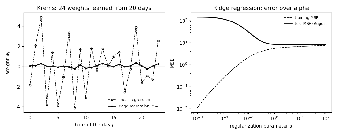
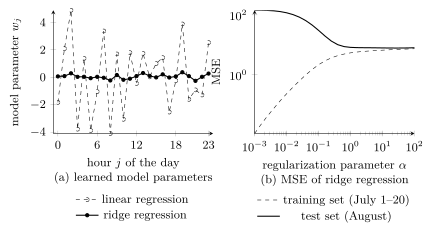
ridgeregression.py, which recomputes what the entry states: the script block by block · open in ColabB-fetchPredicting the maximum temperature of tomorrow at Krems an der Donau from the $24$ hourly temperatures of today is a machine learning (ML) application. A data point is one day, its feature vector ${\mathbf x} \in \mathbb{R}^{24}$ lists the hourly temperatures of the day, and its label $y$ is the maximum temperature of the next day (GeoSphere Austria, 2026). A training set of $m = 20$ days of July 2024 has fewer data points than features, $d = 24$, and the features are nearly collinear: the temperatures at 13:00 and at 14:00 have correlation $0.93$. Linear regression then learns a linear model that reproduces the $20$ training labels exactly and predicts the maximum temperatures of August 2024, the test set, with a mean squared error (MSE) of $141$. Ridge regression learns a linear model from the same training set with a training MSE of $5.4$ and an MSE of $8.3$ on the test set (see Fig. 1).
Ridge regression learns the model parameters ${\mathbf w}$ of a linear hypothesis map $h^{({\mathbf w})}({\mathbf x}) = {\mathbf w}^{\top}{\mathbf x}$, as does linear regression. It minimizes the penalized average squared error loss on a training set $\mathcal{D}^{(\rm train)} = \big\{ \left( {\mathbf x}^{(r)},y^{(r)} \right) \big\}_{r=1}^{m}$ (Hoerl and Kennard, 1970), \begin{equation} \label{eq:ridge_rerm} \widehat{{\mathbf w}}^{(\alpha)} = \mathop{\mathrm{arg\,min}}_{{\mathbf w} \in \mathbb{R}^{d}} \frac{1}{m} \sum_{r=1}^{m} \big( y^{(r)} - {\mathbf w}^{\top}{\mathbf x}^{(r)} \big)^{2} + \alpha \left\lVert {\mathbf w} \right\rVert_{2}^{2} \text{.} \end{equation} The optimization problem can be written more compactly using the feature matrix ${\mathbf X}$ and the label vector ${\mathbf y}$, \[ {\mathbf X} = \big({\mathbf x}^{(1)},\,\ldots,\,{\mathbf x}^{(m)}\big)^{\top} \in \mathbb{R}^{m \times d} \text{,} \qquad {\mathbf y} = \big( y^{(1)},\,\ldots,\,y^{(m)} \big)^{\top} \in \mathbb{R}^{m} \text{.} \] In terms of ${\mathbf X}$ and ${\mathbf y}$, the ridge regression problem \(\eqref{eq:ridge_rerm}\) reads \[ \widehat{{\mathbf w}}^{(\alpha)} = \mathop{\mathrm{arg\,min}}_{{\mathbf w} \in \mathbb{R}^{d}} \frac{1}{m} \left\lVert {\mathbf y} - {\mathbf X} {\mathbf w} \right\rVert_{2}^{2} + \alpha \left\lVert {\mathbf w} \right\rVert_{2}^{2} \text{.} \]
Ridge regression is obtained from linear regression by adding a penalty term to the average squared error loss. The penalty term is the scaled squared Euclidean norm $\alpha \left\lVert {\mathbf w} \right\rVert_{2}^{2}$ with a regularization parameter $\alpha > 0$ (Hastie et al., 2009, Sect. 3.4.1, Eq. (3.41)). The resulting method is an instance of regularized empirical risk minimization (RERM). The purpose of the penalty term is regularization. It prevents overfitting in the high-dimensional regime, where the number of features $d$ exceeds the number of data points $m$ in the training set (Hastie et al., 2009, Sect. 18.1), as it does for the $20$ days with $24$ hourly temperatures each. An alternative method for regularization is least absolute shrinkage and selection operator (Lasso), which differs from ridge regression in the construction of the penalty term: Lasso uses the $\ell_{1}$-norm $\left\lVert {\mathbf w} \right\rVert_{1}$ instead of the squared Euclidean norm $\left\lVert {\mathbf w} \right\rVert_{2}^{2}$.
B-closedIn contrast to Lasso, whose objective can have several minimizers, the ridge regression objective function has, for any feature matrix ${\mathbf X}$ and label vector ${\mathbf y}$, the unique minimizer \begin{equation} \label{eq:ridge_closedform} \widehat{{\mathbf w}}^{(\alpha)} = \big( {\mathbf X}^{\top}{\mathbf X} + \alpha m \mathbf{I} \big)^{-1} {\mathbf X}^{\top}{\mathbf y} \text{.} \end{equation} The normal equations of plain linear regression, by comparison, can have infinitely many solutions, as they do for the $20$ days of July: every one of them reproduces the training labels. Training is a one-shot computation: ridge regression requires no iterative optimization method, and hence no fixed-point interpretation, only the solution of the $d \times d$ system of linear equations $\big( {\mathbf X}^{\top}{\mathbf X} + \alpha m \mathbf{I} \big) {\mathbf w} = {\mathbf X}^{\top}{\mathbf y}$ with an invertible matrix, the zero-gradient condition of the penalized objective function. For many features, gradient descent (GD) on the penalized objective function is the alternative, and the penalty term adds $\alpha m$ to every eigenvalue of ${\mathbf X}^{\top}{\mathbf X}$, which lowers the condition number that sets the convergence rate of GD.
B-svdThe singular value decomposition (SVD) of the feature matrix shows why the linear regression solution amplifies the noise in the labels and how the penalty term bounds the amplification. Write ${\mathbf X} = \mathbf{V} \boldsymbol{\Lambda} \mathbf{U}^{\top}$ with singular values $\lambda_{1} \geq \ldots \geq \lambda_{p} > 0$, where $p$ is the rank of ${\mathbf X}$, with left singular vectors ${\mathbf v}^{(j)}$ and right singular vectors ${\mathbf u}^{(j)}$. The solution of linear regression with the smallest Euclidean norm is \[ \widehat{{\mathbf w}} = \sum_{j=1}^{p} \frac{({\mathbf v}^{(j)})^{\top}{\mathbf y}}{\lambda_{j}} \, {\mathbf u}^{(j)} \text{.} \] Two properties of this solution cause its large test error. A component of ${\mathbf y}$ along ${\mathbf v}^{(j)}$ is divided by $\lambda_{j}$, so a small singular value amplifies the noise in ${\mathbf y}$ by the factor $1/\lambda_{j}$. Small singular values arise from nearly collinear features: the singular values of the $20$ days of hourly temperatures run from $504$ down to $0.21$. And a direction ${\mathbf u}^{(j)}$ with $j > p$, which exists whenever $d > m$, leaves ${\mathbf X} {\mathbf w}$ unchanged, so the training set does not determine the component of ${\mathbf w}$ along it.
B-augInserting the SVD into the closed form \(\eqref{eq:ridge_closedform}\) gives
(Hastie et al., 2009, Sect. 3.4.1, Eq. (3.47))
\[
\widehat{{\mathbf w}}^{(\alpha)} = \sum_{j=1}^{p}
\frac{\lambda_{j}^{2}}{\lambda_{j}^{2}
+ \alpha m} \cdot
\frac{({\mathbf v}^{(j)})^{\top}{\mathbf y}}{\lambda_{j}}
\, {\mathbf u}^{(j)} \text{.}
\]
Ridge regression multiplies each component of
$\widehat{{\mathbf w}}$ in the basis of the right singular
vectors by the shrinkage factor
$\lambda_{j}^{2} / (\lambda_{j}^{2} + \alpha
m)$, which lies strictly between $0$ and $1$. For
$\lambda_{j}^{2} \gg \alpha m$ the factor is
close to $1$ and the component is kept. For
$\lambda_{j}^{2} \ll \alpha m$ the component
is shrunk toward $0$. The product of the factor and
$1/\lambda_{j}$ is
$\lambda_{j} / (\lambda_{j}^{2} + \alpha
m)$, which never exceeds $1/(2\sqrt{\alpha
m})$, so the noise amplification is bounded: for the
$20$ days and $\alpha = 1$, the bound is $0.11$, where
$1/\lambda_{j}$ reaches $4.9$. The undetermined
components with $j > p$ are set to $0$, which is why the
minimizer is unique for any feature matrix. Fig. 1
shows the effect on the learned model parameters: those of
linear regression swing between $-4.1$ and $4.9$ from one hour to the
next, those of ridge regression stay within $\pm 0.4$.
pythondemos/ridgeregression.py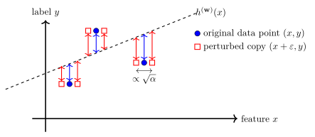
Synonyms: Tikhonov regularization, weight decay.
See also: regression, linear regression, least absolute shrinkage and selection operator, regularization, penalty term, singular value decomposition, condition number, data augmentation, kernel ridge regression.
@misc{dictml_ridgeregression,
  author = {Jung, Alexander},
  editor = {Olioumtsevits, Konstantina and Schnoor, Ekkehard},
  title = {ridge regression},
  howpublished = {Dictionary of Applied Machine Learning (course edition)},
  year = {2026},
  doi = {10.5281/zenodo.21569296},
  note = {ISBN 978-952-64-3013-3, CC BY 4.0, retrieved 2026-11-16},
  url = {https://dictionaryofml.org/terms/ridgeregression.html}
}