Dictionary of Applied Machine Learning
Updated on 2026-10-06
See also empirical risk minimization gradient descent stochastic gradient descent online learning expectation–maximization Gaussian mixture model $k$-means model loss
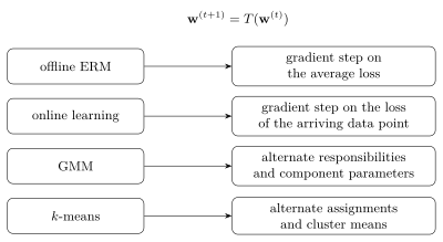
Training is the application of an optimization method to a model, so that its model parameters make a loss computed from data points small. Which method applies is settled by the machine learning (ML) setting rather than by the model alone. Offline empirical risk minimization (ERM) over a fixed training set is solved by gradient descent (GD), or by stochastic gradient descent (SGD) when that training set is large. In online learning, where data points arrive one at a time, online GD takes one step per arriving data point. Unsupervised settings use alternating optimization instead: the expectation–maximization (EM) algorithm trains a Gaussian mixture model (GMM) by alternating between responsibilities and component parameters, and the $k$-means algorithm alternates between cluster assignments and cluster means. All of these iterate a map from the current model parameters to the next, and training stops at or near a fixed point of that map.
Fitting a straight line to a year of electricity records, adapting an hourly forecaster to each new reading as it arrives, and splitting customer profiles into groups are all called training. Each one adjusts the model parameters of a model $\hypospace$ until a loss computed from data points is small. Training is therefore the application of an optimization method, and which method applies is settled by the machine learning (ML) setting rather than by the model alone.
For a parametric model, each hypothesis
$\hypothesis^{(\weights)}$ is fixed by a choice of
model parameters $\weights$, so training searches over $\weights$.
Nearly every method used for that search is an iteration,
\[
\weights^{(\iteridx+1)} = T(\weights^{(\iteridx)})
\text{,}
\]
whose operator $T$ is what changes from one setting to the next.
Training stops at, or near, a fixed point of $T$, where a
further iteration leaves the model parameters unchanged. The
learned hypothesis $\learnthypothesis$ is the one that these
final model parameters define. Four settings and their operators
are collected in Fig. 1.
Unsupervised settings replace the single gradient step by alternating optimization, which splits the model parameters into groups and minimizes over one group while holding the others fixed. Training a Gaussian mixture model (GMM) alternates between the responsibilities of the mixture components for each data point and the parameters of those components, which is the expectation–maximization (EM) algorithm (Dempster et al., 1977). The $k$-means algorithm alternates between assigning each data point to the nearest cluster and recomputing the cluster means (Lloyd, 1982). Both reach a fixed point of their operator, and neither is guaranteed to reach the smallest loss available in $\hypospace$.
The setting therefore decides the method even when the model does not change. A shop forecasts daily bread demand from the weather with a linear model. It trains that linear model by GD on a year of past records. To let the forecaster follow a changing clientele instead, it trains the same linear model by online GD on each new day's sales. One of the main challenges in ML is to control the discrepancy between the loss on the training set and the loss on data points outside it, and no choice of optimization method removes that challenge (Goodfellow et al., 2016).
Synonyms: model fitting, fitting.
See also: optimization problem, empirical risk minimization, gradient descent, stochastic gradient descent, online learning, expectation–maximization, Gaussian mixture model, $k$-means, fixed point, model, model parameter, loss.
@misc{dictml_training,
  author = {Jung, Alexander},
  editor = {Olioumtsevits, Konstantina and Schnoor, Ekkehard},
  title = {training},
  howpublished = {Dictionary of Applied Machine Learning (course edition)},
  year = {2026},
  doi = {10.5281/zenodo.21569296},
  note = {ISBN 978-952-64-3013-3, CC BY 4.0, retrieved 2026-10-06},
  url = {https://dictionaryofml.org/terms/training.html}
}