correlation.py, which recomputes what the entry states: the script block by block · open in ColabDictionary of Applied Machine Learning: 114 machine-learning terms, each with a definition, a figure, citations and a Python demo · All terms · Demos · Start here
Updated on 2026-11-01
Readiness 80/100
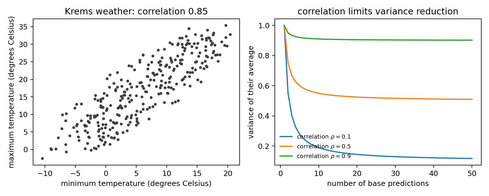
Correlation measures the strength and direction of the linear relationship between two real-valued random variables (RVs). It is obtained by normalizing their covariance by their standard deviations, making it dimensionless and comparable across quantities measured on different scales. Its extreme positive and negative values characterize perfect increasing and decreasing affine relationships, while its central value characterizes uncorrelated variables. Independent RVs are uncorrelated, but uncorrelated RVs need not be independent, since correlation quantifies only linear dependence. The correlation between the predictions of the base learners of an ensemble bounds the variance reduction that averaging them can achieve.
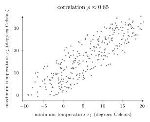
correlation.py, which recomputes what the entry states: the script block by block · open in ColabB-dataFig. 1 shows a dataset that consists of $1827$ daily weather measurements at Krems an der Donau. Each data point represents a day, characterized by the minimum and the maximum temperature as its feature vector ${\mathbf x}=(x_{1},x_{2})^{\top}$. Selecting a data point from the dataset uniformly at random defines a random vector ${\mathbf x}$. Correlation quantifies whether a day whose minimum temperature is unusually high also tends to have an unusually high maximum temperature.
B-corrMore generally, for two real-valued random variables (RVs) $x$ and $y$ on a common probability space with nonzero standard deviations $\sigma_{x}$ and $\sigma_{y}$, their correlation is their covariance normalized by the product of these standard deviations (Bertsekas and Tsitsiklis, 2008), \[ \rho := \frac{{\rm cov}\left(x,y\right)}{\sigma_{x}\,\sigma_{y}} \in [-1, 1]\text{.} \] The value $\rho$ is also referred to as the Pearson correlation coefficient.
B-figUnlike the covariance, correlation is dimensionless. Adding a
constant to either RV, or multiplying it by a positive constant,
does not change $\rho$; multiplying one RV by a negative constant
reverses its sign
(Anderson, 2003, Sec. 2.3, Thm. 2.3.2).
The extreme values $\rho = 1$
and $\rho = -1$ occur exactly when $y$ is an increasing or a
decreasing affine function of $x$ with probability
one (Meyer, 2000, Sec. 5.4). The RVs are
uncorrelated when $\rho = 0$ (Bertsekas and Tsitsiklis, 2008, Sec. 4.2).
Independent RVs are uncorrelated, but uncorrelated
RVs need not be independent, since $\rho$ quantifies only
linear dependence (Bertsekas and Tsitsiklis, 2008, Sec. 4.2). For the
random vector ${\mathbf x}$ obtained by selecting uniformly at
random one of the daily minimum-and-maximum temperature pairs shown in
Fig. 1, the covariance between the two
temperatures is $55.08$ squared degrees Celsius, and their variances
are $49.89$ and $83.41$ squared degrees Celsius. Thus,
\[
\rho = \frac{55.08}{\sqrt{49.89\cdot83.41}} \approx 0.85\text{.}
\]
pythondemos/correlation.py
@misc{dictml_correlation,
  author = {Jung, Alexander},
  editor = {Olioumtsevits, Konstantina and Schnoor, Ekkehard},
  title = {correlation},
  howpublished = {Dictionary of Applied Machine Learning (course edition)},
  year = {2026},
  doi = {10.5281/zenodo.21569296},
  note = {ISBN 978-952-64-3013-3, CC BY 4.0, retrieved 2026-11-02},
  url = {https://dictionaryofml.org/terms/correlation.html}
}