B-fig writes when the script runsDictionary of Applied Machine Learning · correlation
Updated on 2026-11-01
Numerical companion to the entry correlation: it recomputes what the entry states and prints one line per check
Correlation is covariance normalized by the standard deviations. This demo constructs the weather random vector used in the entry from 1827 daily measurements at Krems an der Donau, computes its correlation, and checks the entry's interpretation and invariance claims. It also constructs dependent but uncorrelated random variables and verifies the variance formula that explains why correlated base predictions limit an ensemble's benefit.
Run it without installing anything:uv run https://dictionaryofml.org/terms/correlation.py
uv downloads this script and the pinned NumPy and Matplotlib it needs, then runs it; the script fetches any input file it uses. To keep the output files, download correlation.py into a folder and run uv run correlation.py there. With NumPy and Matplotlib already installed, python3 correlation.py, from any directory — it writes its output files into the current directory. Fixed seeds, so the printed numbers reproduce exactly. Download correlation.py · Notebook · Open in Colab
One cell per block of the script: the code, and what that code printed when it last ran here
"""Numerical companion to the glossary entry 'correlation'.

Purpose
-------
Correlation is covariance normalized by the standard deviations. This demo
constructs the weather random vector used in the entry from 1827 daily
measurements at Krems an der Donau, computes its correlation, and checks the
entry's interpretation and invariance claims. It also constructs dependent
but uncorrelated random variables and verifies the variance formula that
explains why correlated base predictions limit an ensemble's benefit.

Self-contained (NumPy + Matplotlib only, with stdlib urllib for the weather
archive). The synthetic experiments use a fixed random seed.

Blocks
------
[B-data]     Download daily minimum and maximum temperatures for 2020--2024.
[B-corr]     Compute normalized covariance and write the plotted datapoints.
[B-scale]    Check the effects of shifts and positive or negative scaling.
[B-depend]   Exhibit dependent but uncorrelated variables Z and Z squared.
[B-ensemble] Verify the variance of equicorrelated averaged predictions.
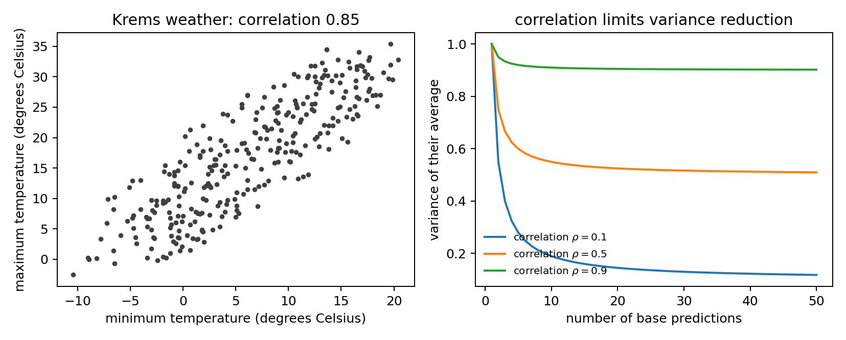
[B-fig]      Plot the weather datapoints and ensemble variance curves.

Outputs
-------
correlation_days_plot.csv         : every sixth weather datapoint
correlation_ensemble_variance.csv : ensemble size and theoretical variances
correlation.png                   : preview of both experiments
"""

import json
import urllib.request
from pathlib import Path

import matplotlib
import numpy as np

matplotlib.use("Agg")
import matplotlib.pyplot as plt

OUT_DIR = Path(__file__).parent
ARCHIVE = "https://dataset.api.hub.geosphere.at/v1/station/historical/"
STATION = 3805
EVERY = 6
rng = np.random.default_rng(20261101)
report = []


def check(name, condition):
    report.append((name, bool(condition)))
    print(f"  [{'ok' if condition else 'FAIL'}] {name}")


def correlation(x, y):
    centered_x = x - x.mean()
    centered_y = y - y.mean()
    covariance = np.mean(centered_x * centered_y)
    return covariance / np.sqrt(np.mean(centered_x**2) *
                                np.mean(centered_y**2))
Download daily minimum and maximum temperatures for 2020--2024.
url = (f"{ARCHIVE}klima-v2-1d?parameters=tlmin,tlmax"
       f"&station_ids={STATION}&start=2020-01-01&end=2024-12-31")
with urllib.request.urlopen(url, timeout=240) as response:
    payload = json.load(response)
values = payload["features"][0]["properties"]["parameters"]
days = np.column_stack((np.asarray(values["tlmin"]["data"], dtype=float),
                        np.asarray(values["tlmax"]["data"], dtype=float)))
check("[B-data] 1827 daily weather datapoints were downloaded without gaps",
      days.shape == (1827, 2) and np.all(np.isfinite(days)))
[ok] [B-data] 1827 daily weather datapoints were downloaded without gaps
Compute normalized covariance and write the plotted datapoints.
centered = days - days.mean(axis=0)
covariance_matrix = centered.T @ centered / len(days)
rho = (covariance_matrix[0, 1] /
       np.sqrt(covariance_matrix[0, 0] * covariance_matrix[1, 1]))
check("[B-corr] normalized covariance equals direct correlation",
      np.isclose(rho, correlation(days[:, 0], days[:, 1])))
check("[B-corr] Krems temperatures have correlation about 0.85",
      np.isclose(rho, 0.854, atol=0.001))

plot_days = days[::EVERY]
with open(OUT_DIR / "correlation_days_plot.csv", "w") as stream:
    stream.write("tmin,tmax\n")
    for tmin, tmax in plot_days:
        stream.write(f"{tmin:.3f},{tmax:.3f}\n")
check("[B-corr] the scatter contains every sixth day", len(plot_days) == 305)
  [ok] [B-corr] normalized covariance equals direct correlation
  [ok] [B-corr] Krems temperatures have correlation about 0.85
  [ok] [B-corr] the scatter contains every sixth day
Check the effects of shifts and positive or negative scaling.
x, y = days[:, 0], days[:, 1]
check("[B-scale] shifts and positive scaling leave correlation unchanged",
      np.isclose(correlation(3.0 * x + 7.0, 0.5 * y - 4.0), rho))
check("[B-scale] negative scaling reverses the sign",
      np.isclose(correlation(-x, y), -rho))
check("[B-scale] an increasing affine relation has correlation 1",
      np.isclose(correlation(x, 2.5 * x - 3.0), 1.0))
check("[B-scale] a decreasing affine relation has correlation -1",
      np.isclose(correlation(x, -2.5 * x - 3.0), -1.0))
  [ok] [B-scale] shifts and positive scaling leave correlation unchanged
  [ok] [B-scale] negative scaling reverses the sign
  [ok] [B-scale] an increasing affine relation has correlation 1
  [ok] [B-scale] a decreasing affine relation has correlation -1
Exhibit dependent but uncorrelated variables Z and Z squared.
z = rng.uniform(-1.0, 1.0, 200_000)
z_squared = z**2
rho_dependent = correlation(z, z_squared)
check("[B-depend] Z and Z squared are approximately uncorrelated",
      abs(rho_dependent) < 0.01)
check("[B-depend] but Z squared is completely determined by Z",
      np.allclose(z_squared, z**2))
  [ok] [B-depend] Z and Z squared are approximately uncorrelated
  [ok] [B-depend] but Z squared is completely determined by Z
Verify the variance of equicorrelated averaged predictions.
ensemble_sizes = np.arange(1, 51)
correlations = (0.1, 0.5, 0.9)
variance_curves = {
    r: r + (1.0 - r) / ensemble_sizes for r in correlations
}
for r, curve in variance_curves.items():
    covariance = np.full((8, 8), r)
    np.fill_diagonal(covariance, 1.0)
    exact = np.ones(8) @ covariance @ np.ones(8) / 8**2
    check(f"[B-ensemble] averaging formula holds for rho={r:.1f}",
          np.isclose(exact, curve[7]))

with open(OUT_DIR / "correlation_ensemble_variance.csv", "w") as stream:
    stream.write("learners,rho_01,rho_05,rho_09\n")
    for i, learners in enumerate(ensemble_sizes):
        stream.write(f"{learners},{variance_curves[0.1][i]:.6f},"
                     f"{variance_curves[0.5][i]:.6f},"
                     f"{variance_curves[0.9][i]:.6f}\n")
  [ok] [B-ensemble] averaging formula holds for rho=0.1
  [ok] [B-ensemble] averaging formula holds for rho=0.5
  [ok] [B-ensemble] averaging formula holds for rho=0.9
  wrote /Users/junga1/dictionaryappliedml/pythondemos/correlation.png

13/13 checks pass.
Plot the weather datapoints and ensemble variance curves.
fig, axes = plt.subplots(1, 2, figsize=(9.2, 3.7))
axes[0].scatter(plot_days[:, 0], plot_days[:, 1], s=8, color="0.25")
axes[0].set_xlabel("minimum temperature (degrees Celsius)")
axes[0].set_ylabel("maximum temperature (degrees Celsius)")
axes[0].set_title(f"Krems weather: correlation {rho:.2f}")

for r, curve in variance_curves.items():
    axes[1].plot(ensemble_sizes, curve, lw=1.6,
                 label=rf"correlation $\rho={r:.1f}$")
axes[1].set_xlabel("number of base predictions")
axes[1].set_ylabel("variance of their average")
axes[1].set_title("correlation limits variance reduction")
axes[1].legend(frameon=False, fontsize=8)
fig.tight_layout()
fig.savefig(OUT_DIR / "correlation.png", dpi=180)
print(f"  wrote {OUT_DIR / 'correlation.png'}")

n_fail = sum(not passed for _, passed in report)
print(f"\n{len(report) - n_fail}/{len(report)} checks pass.")
raise SystemExit(1 if n_fail else 0)
B-fig writes when the script runs