Dictionary of Applied Machine Learning
Updated on 2026-10-08
See also dataset data point feature vector feature matrix singular value decomposition principal component analysis dimensionality reduction
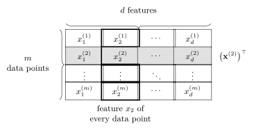
The feature matrix of a dataset collects the feature vectors of its data points as its rows, so it has one row per data point and one column per feature. Reading it along a row returns one data point, and reading it along a column returns one feature across the whole dataset. A few numbers computed from it summarize the dataset. Its shape is the pair of the number of data points and the number of features, and linear regression has a unique solution only when the feature matrix has full column rank. Its singular values are at most as many numbers as its smaller dimension, the count of the nonzero ones is its rank, and their squares are the eigenvalues of $\featuremtx^{\top} \featuremtx$, which divided by the number of data points is the sample covariance matrix. The condition number, the ratio of the largest singular value to the smallest nonzero one, bounds how far the linear regression solution moves when the labels are perturbed.
A weather station at Krems an der Donau records eight measurements on each day of a year: the lowest, highest and mean air temperature, the precipitation, the sunshine duration, the humidity, the air pressure and the wind speed. Writing the eight measurements of one day as a row, and placing the rows of the $366$ days under one another, gives a table of numbers. That table is the feature matrix of the dataset.
B-shapeConsider a dataset $\dataset$
of $\samplesize$ data points with feature vectors
$\featurevec^{(1)}, \,\ldots, \,\featurevec^{(\samplesize)}$, each in
$\reals^{\nrfeatures}$.
It is convenient to collect the individual feature vectors into
the feature matrix:
\[\featuremtx \defeq \big(\featurevec^{(1)}, \,\ldots, \,\featurevec^{(\samplesize)}\big)^{\top} =
\begin{pmatrix}
\feature^{(1)}_{1} & \feature^{(1)}_{2} & \cdots & \feature^{(1)}_{\nrfeatures} \\
\feature^{(2)}_{1} & \feature^{(2)}_{2} & \cdots & \feature^{(2)}_{\nrfeatures} \\
\vdots & \vdots & \ddots & \vdots \\
\feature^{(\samplesize)}_{1} & \feature^{(\samplesize)}_{2} & \cdots & \feature^{(\samplesize)}_{\nrfeatures}
\end{pmatrix}
\in \reals^{\samplesize \times \nrfeatures} \text{.}\]
Note that the feature matrix is of size $\samplesize \times \nrfeatures$, i.e.,
it has $\samplesize$ rows and $\nrfeatures$ columns. Each row holds one
data point and each column holds one feature, so reading the
feature matrix along a row or along a column answers two
different questions (see Fig. 1).
B-spectrumThe next summaries come from the singular value decomposition (SVD) of $\featuremtx$. Its singular values $\eigval{1} \geq \ldots \geq \eigval{\min\{\samplesize, \nrfeatures\}} \geq 0$ are at most $\min\{\samplesize, \nrfeatures\}$ numbers, and the count of the nonzero ones is the rank of $\featuremtx$ (Golub and Loan, 2013, Sect. 2.4). A rank below $\nrfeatures$ means that some feature is a linear combination of the others and carries nothing new. The squares of the singular values are the eigenvalues of $\featuremtx^{\top} \featuremtx$, and this matrix divided by $\samplesize$ is the sample covariance matrix of features with zero sample mean. The spectrum is therefore what principal component analysis (PCA) uses to decide how many features a dimensionality reduction can keep.
One number summarizes how far apart the singular values lie, the condition number $\condnumber{\featuremtx} = \eigval{1} / \eigval{\operatorname{rank}(\featuremtx)}$. It is the ratio of the largest singular value to the smallest nonzero one. It bounds how far the linear regression solution moves when the labels are perturbed, and it governs how fast gradient descent (GD) converges on the least squares objective function (Boyd and Vandenberghe, 2004, Sect. 9.3).
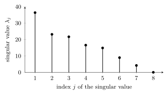
Fig. 2 shows these summaries for the weather year at Krems an der Donau. Each data point is a day and carries the eight measurements as its features, so the feature matrix is of shape $(366, 8)$ and holds $2928$ numbers. Each feature is first scaled to zero sample mean and unit sample variance, because the measurements carry different units. Eight singular values then summarize the whole year: the largest is $36.4$ and the smallest $0.05$, the two largest carry $64$ percent of the sum of the squared singular values, and the four largest carry $89$ percent.
B-condThe smallest singular value lies far below the others, and it
names a redundancy among the features. The mean temperature of
a day differs from the midpoint of its lowest and its highest
temperature by $0.02$ degrees Celsius on average. Dropping the mean
temperature raises the smallest singular value to $4.19$ and
lowers the condition number from $748$ to $7.6$. The rank is $8$
either way, so the rank alone does not see this near-dependency
and the singular values do.
pythondemos/featuremtx.py
See also: dataset, data point, feature vector, feature, matrix, singular value decomposition, singular value, rank, condition number, spectrum, sample covariance matrix, principal component analysis, dimensionality reduction.
@misc{dictml_featuremtx,
  author = {Jung, Alexander},
  editor = {Olioumtsevits, Konstantina and Schnoor, Ekkehard},
  title = {feature matrix},
  howpublished = {Dictionary of Applied Machine Learning (course edition)},
  year = {2026},
  doi = {10.5281/zenodo.21569296},
  note = {ISBN 978-952-64-3013-3, CC BY 4.0, retrieved 2026-10-08},
  url = {https://dictionaryofml.org/terms/featuremtx.html}
}