B-fig writes when the script runsDictionary of Applied Machine Learning · feature matrix
Numerical companion to the entry feature matrix: it recomputes what the entry states and prints one line per check
Numerical companion to the glossary entry 'featuremtx'. The GeoSphere Austria weather station Krems (station id 3805) records eight measurements per day: minimum, maximum and mean air temperature, precipitation, sunshine duration, relative humidity, air pressure and wind speed. This script downloads the records for 2024 from the GeoSphere data hub (dataset klima-v2-1d) and writes them to featuremtx_weather.csv. A value of -1 for precipitation marks a trace of rain too small to record and is set to 0.
Run it without installing anything:uv run https://dictionaryofml.org/terms/featuremtx.py
uv downloads this script and the pinned NumPy and Matplotlib it needs, then runs it; the script fetches any input file it uses. To keep the output files, download featuremtx.py into a folder and run uv run featuremtx.py there. With NumPy and Matplotlib already installed, python3 featuremtx.py, from any directory — it writes its output files into the current directory. Fixed seeds, so the printed numbers reproduce exactly. Download featuremtx.py · Notebook · Open in Colab
One cell per block of the script: the code, and what that code printed when it last ran here
"""The feature matrix of one weather year, summarized by a handful of
numbers: its shape, its rank, its singular values and its condition number.

Purpose
-------
Numerical companion to the glossary entry 'featuremtx'.  The GeoSphere
Austria weather station Krems (station id 3805) records eight
measurements per day: minimum, maximum and mean air temperature,
precipitation, sunshine duration, relative humidity, air pressure and
wind speed.  This script downloads the records for 2024 from the
GeoSphere data hub (dataset klima-v2-1d) and writes them to
featuremtx_weather.csv.  A value of -1 for precipitation marks a trace
of rain too small to record and is set to 0.

Collecting the eight measurements of each day as a row gives the feature
matrix of the year.  Every measurement is scaled to zero sample mean and
unit sample variance first, because temperatures, precipitation and
pressure carry different units and the singular values of an unscaled
matrix would report the choice of units rather than the data.

The demo checks the claims the entry makes.  (1) The shape is the pair
(number of data points, number of features), and the whole year is 366
times 8 numbers while the shape is two of them.  (2) The singular values
are the square roots of the eigenvalues of X^T X, and X^T X divided by
the number of data points is the sample covariance matrix of the scaled
measurements, so the singular values carry the spectrum that PCA reads.
(3) The sum of the squared singular values is the squared Frobenius norm
of the feature matrix, which for scaled measurements is the number of
data points times the number of features.  (4) The condition number is
the ratio of the largest to the smallest singular value.  (5) The
smallest singular value is far below the largest because the mean
temperature of a day is close to the midpoint of its minimum and its
maximum, a near-dependency among three columns; dropping the mean
temperature raises the smallest singular value by more than an order of
magnitude.

Deterministic: the data are a fixed archive year and the decomposition
is a singular value decomposition.  Self-contained: numpy + matplotlib
only (stdlib urllib for the download).

Blocks
------
[B-data]      Download the 366 days with eight measurements each and
              scale every measurement to zero sample mean and unit
              sample variance.
[B-shape]     The shape of the feature matrix, and how many numbers it
              takes to state it.
[B-spectrum]  The singular values, their link to the eigenvalues of
              X^T X and to the sample covariance matrix, and the share
              of the squared Frobenius norm that the leading ones carry.
[B-cond]      The rank and the condition number, and the near-dependency
              among the three temperature columns that makes the
              smallest singular value small.
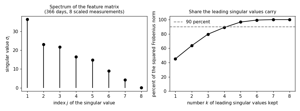
[B-fig]       The preview figure: the spectrum as a stem plot and the
              share of the squared Frobenius norm that k singular values
              carry.

Outputs
-------
featuremtx_weather.csv   : date and the eight measurements, 366 days
featuremtx_spectrum.csv  : index, singular value, cumulative share
featuremtx.png           : preview figure
"""

import json
import urllib.request
from pathlib import Path

import matplotlib
matplotlib.use("Agg")
import matplotlib.pyplot as plt                        # noqa: E402
import numpy as np                                     # noqa: E402

OUT_DIR = Path(__file__).parent

FAILED = []


def check(name, ok):
    FAILED.append(name) if not ok else None
    print(f"  [{'ok' if ok else 'FAIL'}] {name}")
Download the 366 days with eight measurements each and scale every measurement to zero sample mean and unit sample variance.
PARAMS = ["tlmin", "tlmax", "tl_mittel", "rr", "so_h", "rf_mittel",
          "p_mittel", "vv_mittel"]
URL = ("https://dataset.api.hub.geosphere.at/v1/station/historical/"
       f"klima-v2-1d?parameters={','.join(PARAMS)}&station_ids=3805"
       "&start=2024-01-01&end=2024-12-31")
with urllib.request.urlopen(URL, timeout=180) as resp:
    payload = json.load(resp)
params = payload["features"][0]["properties"]["parameters"]
stamps = [t[:10] for t in payload["timestamps"]]
RAW = np.stack([np.array(params[p]["data"], dtype=float) for p in PARAMS], 1)
RAW[:, 3] = np.maximum(RAW[:, 3], 0.0)       # -1 marks a trace of rain
with open(OUT_DIR / "featuremtx_weather.csv", "w") as f:
    f.write("date," + ",".join(PARAMS) + "\n")
    for day, row in zip(stamps, RAW):
        f.write(day + "," + ",".join(f"{v:g}" for v in row) + "\n")

X = (RAW - RAW.mean(0)) / RAW.std(0)         # zero mean, unit variance
print("[B-data] the feature matrix of one weather year")
check("[B-data] every measurement has zero sample mean and unit variance",
      np.allclose(X.mean(0), 0.0, atol=1e-12)
      and np.allclose(X.std(0), 1.0, atol=1e-12))
[B-data] the feature matrix of one weather year
  [ok] [B-data] every measurement has zero sample mean and unit variance
The shape of the feature matrix, and how many numbers it takes to state it.
m, d = X.shape
print(f"[B-shape] shape ({m}, {d}): {m} data points, {d} features")
print(f"[B-shape] {m * d} numbers in the matrix, 2 in its shape")
check("[B-shape] 366 days with eight measurements each",
      (m, d) == (366, 8))
check("[B-shape] more data points than features", m > d)
[B-shape] shape (366, 8): 366 data points, 8 features
[B-shape] 2928 numbers in the matrix, 2 in its shape
  [ok] [B-shape] 366 days with eight measurements each
  [ok] [B-shape] more data points than features
The singular values, their link to the eigenvalues of X^T X and to the sample covariance matrix, and the share of the squared Frobenius norm that the leading ones carry.
sv = np.linalg.svd(X, compute_uv=False)
eigs = np.linalg.eigvalsh(X.T @ X)[::-1]
cum = np.cumsum(sv ** 2) / np.sum(sv ** 2)
print("[B-spectrum] singular values: "
      + ", ".join(f"{s:.2f}" for s in sv))
print(f"[B-spectrum] two of them carry {100 * cum[1]:.0f}% of the "
      f"squared Frobenius norm, four carry {100 * cum[3]:.0f}%")
check("[B-spectrum] the squared singular values are the eigenvalues "
      "of X^T X", np.allclose(sv ** 2, eigs, rtol=1e-9, atol=1e-9))
samplecov = (X.T @ X) / m
check("[B-spectrum] X^T X divided by the number of data points is the "
      "sample covariance matrix of the scaled measurements",
      np.allclose(samplecov, np.cov(X, rowvar=False, bias=True),
                  atol=1e-12))
check("[B-spectrum] the squared singular values sum to the squared "
      "Frobenius norm, which is m times d here",
      abs(np.sum(sv ** 2) - m * d) < 1e-6)
with open(OUT_DIR / "featuremtx_spectrum.csv", "w") as f:
    f.write("j,sigma,share\n")
    for j, (s, c) in enumerate(zip(sv, cum), start=1):
        f.write(f"{j},{s:.6f},{c:.6f}\n")
[B-spectrum] singular values: 36.40, 23.17, 21.69, 16.58, 14.89, 8.99, 4.23, 0.05
[B-spectrum] two of them carry 64% of the squared Frobenius norm, four carry 89%
  [ok] [B-spectrum] the squared singular values are the eigenvalues of X^T X
  [ok] [B-spectrum] X^T X divided by the number of data points is the sample covariance matrix of the scaled measurements
  [ok] [B-spectrum] the squared singular values sum to the squared Frobenius norm, which is m times d here
The rank and the condition number, and the near-dependency among the three temperature columns that makes the smallest singular value small.
rank = int(np.linalg.matrix_rank(X))
cond = sv[0] / sv[-1]
print(f"[B-cond] rank {rank}, condition number {cond:.1f}")
check("[B-cond] the rank is the number of features, so no measurement "
      "is an exact combination of the others", rank == d)
check("[B-cond] the condition number is the ratio of the largest to "
      "the smallest singular value",
      abs(cond - np.linalg.cond(X)) < 1e-6)
# the mean temperature is close to the midpoint of the extremes
mid = 0.5 * (RAW[:, 0] + RAW[:, 1])
gap = np.abs(RAW[:, 2] - mid)
print(f"[B-cond] mean temperature differs from the midpoint of the "
      f"extremes by {gap.mean():.2f} degrees on average")
keep = [i for i in range(d) if i != 2]            # drop mean temperature
sv_keep = np.linalg.svd(X[:, keep], compute_uv=False)
cond_keep = sv_keep[0] / sv_keep[-1]
print(f"[B-cond] dropping the mean temperature: smallest singular value "
      f"{sv[-1]:.2f} -> {sv_keep[-1]:.2f}, condition number "
      f"{cond:.1f} -> {cond_keep:.1f}")
check("[B-cond] dropping the mean temperature raises the smallest "
      "singular value by more than an order of magnitude",
      sv_keep[-1] > 10 * sv[-1])
check("[B-cond] and lowers the condition number by more than an order "
      "of magnitude", cond_keep < cond / 10)
[B-cond] rank 8, condition number 748.0
  [ok] [B-cond] the rank is the number of features, so no measurement is an exact combination of the others
  [ok] [B-cond] the condition number is the ratio of the largest to the smallest singular value
[B-cond] mean temperature differs from the midpoint of the extremes by 0.02 degrees on average
[B-cond] dropping the mean temperature: smallest singular value 0.05 -> 4.19, condition number 748.0 -> 7.6
  [ok] [B-cond] dropping the mean temperature raises the smallest singular value by more than an order of magnitude
  [ok] [B-cond] and lowers the condition number by more than an order of magnitude
The preview figure: the spectrum as a stem plot and the share of the squared Frobenius norm that k singular values carry.
fig, (axL, axR) = plt.subplots(1, 2, figsize=(9.4, 3.5))
axL.stem(np.arange(1, d + 1), sv, linefmt="k-", markerfmt="ko",
         basefmt=" ")
axL.set_xlabel("index $j$ of the singular value")
axL.set_ylabel("singular value $\\sigma_j$")
axL.set_title("Spectrum of the feature matrix\n(366 days, 8 scaled "
              "measurements)", fontsize=10)
axL.set_xticks(np.arange(1, d + 1))
axR.plot(np.arange(1, d + 1), 100 * cum, "k-o")
axR.axhline(90, color="gray", linestyle="--", label="90 percent")
axR.set_xlabel("number $k$ of leading singular values kept")
axR.set_ylabel("percent of the squared Frobenius norm")
axR.set_title("Share the leading singular values carry", fontsize=10)
axR.set_xticks(np.arange(1, d + 1))
axR.set_ylim(0, 105)
axR.legend(frameon=False)
fig.tight_layout()
fig.savefig(OUT_DIR / "featuremtx.png", dpi=110)
check("[B-fig] the preview figure was written",
      (OUT_DIR / "featuremtx.png").exists())

print()
if FAILED:
    print(f"{len(FAILED)} check(s) FAILED: " + "; ".join(FAILED))
    raise SystemExit(1)
print("all checks passed")
  [ok] [B-fig] the preview figure was written

all checks passed
B-fig writes when the script runs