pythondemos/dataaug.pyDictionary of Applied Machine Learning
Updated on 2026-10-08
See also regularization overfitting empirical risk minimization training set hypothesis space data point label feature vector
Data augmentation enlarges a training set with synthetic data points obtained by perturbing or transforming the measured ones. It is one of the three routes that regularization distinguishes, beside shrinking the hypothesis space and adding a penalty term. A perturbation is admissible when it is known to leave the label alone, either because the feature space carries a symmetry, such as the rotation of an image, or because the measurement is only accurate to within a stated tolerance. Enlarging the training set this way removes hypothesis maps that the training error alone cannot rule out, since a copy displaced along the feature axis misses its label whenever the hypothesis is steep there. For the squared error loss, perturbing the features with noise is equivalent to adding a penalty term that grows with the noise variance, which is why the three routes often coincide.
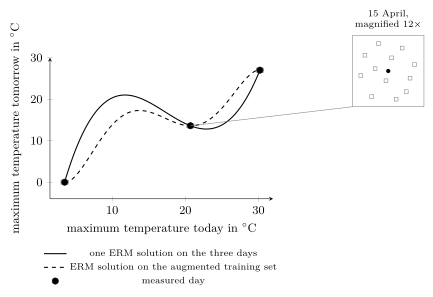
A weather station at Krems an der Donau measured a maximum temperature of $3.5\,^{\circ}$C on 21 January 2024, $20.7\,^{\circ}$C on 15 April and $30.2\,^{\circ}$C on 19 July. On the day after each of them it measured $0.0$, $13.6$ and $27.0\,^{\circ}$C. Take these three days as a training set for predicting tomorrow's maximum temperature from today's, and let the hypothesis space be the polynomials of degree five (see polynomial regression).
B-overfitA polynomial of degree five carries six model parameters and the training set holds three data points, so empirical risk minimization (ERM) has infinitely many solutions. Three independent directions change the polynomial without moving it at the three measured temperatures, so every solution has a training error of zero and the training error cannot choose among them. Between the measured days the solutions take every value: at a today-maximum of $12\,^{\circ}$C the smoothest of them predicts $6.8\,^{\circ}$C for tomorrow, while the solution drawn in Fig. 1 predicts $21.0\,^{\circ}$C. The two differ by up to $15\,^{\circ}$C between the measured days. This is overfitting: the hypothesis space is too large for three data points.
B-augmentWhat rules the wild solutions out is something the thermometer already says. It reports the air temperature only to within its accuracy, taken here to be $0.5\,^{\circ}$C. Both the feature and the label of one of these data points are readings of that instrument, so a day whose two numbers are moved anywhere inside that tolerance is just as consistent with what was measured. Replacing each measured day by copies drawn that way gives an augmented training set (the open squares in Fig. 1). The perturbation is justified by the instrument, not invented: it asserts only that the labels of two days whose readings agree to within the sensor accuracy should agree too, which is the smoothness assumption read at the scale of the measurement error.
B-compareThe copies carry many distinct features, so the
feature matrix of the augmented training set has full column
rank and ERM on it has a unique solution. A polynomial
that is steep where the copies lie pays for that steepness, because a
copy displaced along the feature axis then misses its
label. On the $309$ days of 2024 that were held out and whose
today-maximum lies between $3.5$ and $30.2\,^{\circ}$C, the solution
drawn in Fig. 1 incurs an average
squared error loss of $71.8$ squared degrees. The solution on the
augmented training set incurs $32.6$, against $30.9$ for the
straight line through the three measured days.
pythondemos/dataaug.py
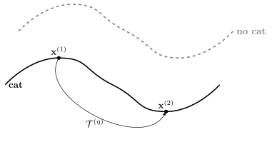
When the features are perturbed, the operation is chosen so
that the synthetic data points keep the same label. An
operator that maps the feature space $\featurespace$
into itself and is known to leave the label alone is called a
symmetry of the learning task. For example, a rotated cat image still shows
a cat, while its
feature vector (obtained by stacking pixel color intensities)
differs from that of the original image (see Fig. 2).
See also: regularization, overfitting, empirical risk minimization, training set, penalty term, hypothesis space, data point, label, feature vector, feature space, smoothness assumption, polynomial regression, ridge regression.
@misc{dictml_dataaug,
  author = {Jung, Alexander},
  editor = {Olioumtsevits, Konstantina and Schnoor, Ekkehard},
  title = {data augmentation},
  howpublished = {Dictionary of Applied Machine Learning (course edition)},
  year = {2026},
  doi = {10.5281/zenodo.21569296},
  note = {ISBN 978-952-64-3013-3, CC BY 4.0, retrieved 2026-10-08},
  url = {https://dictionaryofml.org/terms/dataaug.html}
}