B-figure writes when the script runsDictionary of Applied Machine Learning · ridge regression
Updated on 2026-11-16
Numerical companion to the entry ridge regression: it recomputes what the entry states and prints one line per check
Ridge regression learns the parameters w of a linear hypothesis by minimizing the average squared error loss on a trainset plus the penalty term alpha ||w||_2^2; its unique minimizer is w_hat = (X^T X + alpha m I)^{-1} X^T y for ANY feature matrix X. The demo runs the method on the entry's application, predicting the maximum temperature of the next day at Krems an der Donau from the 24 hourly temperatures of a day with fewer training days than features, and verifies the entry's claims: the closed form, the failure of plain linear regression when m < d, the SVD shrinkage view with its bound on the noise amplification, the condition number of the penalized normal equations, and the data augmentation interpretation (Bishop 1995). Self-contained (numpy/matplotlib only), fixed seed; the weather data is downloaded from the GeoSphere Austria archive.
Run it without installing anything:uv run https://dictionaryofml.org/terms/ridgeregression.py
uv downloads this script and the pinned NumPy and Matplotlib it needs, then runs it; the script fetches any input file it uses. To keep the output files, download ridgeregression.py into a folder and run uv run ridgeregression.py there. With NumPy and Matplotlib already installed, python3 ridgeregression.py, from any directory — it writes its output files into the current directory. Fixed seeds, so the printed numbers reproduce exactly. Download ridgeregression.py · Notebook · Open in Colab
Before running a downloaded copy, scan it: uvx bandit -q -t B102,B307,B602,B605 ridgeregression.py (B102,B307,B602,B605 are the exec, eval and shell checks of bandit) reports nothing: the script runs no shell command and evaluates no generated code.
One cell per block of the script: the code, and what that code printed when it last ran here
"""
ridgeregression.py — numerical companion to the glossary entry
'ridge regression'.

Purpose
-------
Ridge regression learns the parameters w of a linear hypothesis by
minimizing the average squared error loss on a trainset plus the penalty
term alpha ||w||_2^2; its unique minimizer is w_hat = (X^T X + alpha m
I)^{-1} X^T y for ANY feature matrix X.  The demo runs the method on the
entry's application, predicting the maximum temperature of the next day
at Krems an der Donau from the 24 hourly temperatures of a day with
fewer training days than features, and verifies the entry's claims:
the closed form, the failure of plain linear regression when m < d, the
SVD shrinkage view with its bound on the noise amplification, the
condition number of the penalized normal equations, and the data
augmentation interpretation (Bishop 1995).  Self-contained
(numpy/matplotlib only), fixed seed; the weather data is downloaded from
the GeoSphere Austria archive.

Blocks
------
[B-fetch]    Hourly air temperature (klima-v2-1h, tl) and daily maximum
             temperature (klima-v2-1d, tlmax) at Krems an der Donau,
             GeoSphere station 3805, July and August 2024.  A data point
             is one day: feature vector x = its 24 hourly temperatures
             (d = 24), label y = the maximum temperature of the next day.
             Trainset: July 1 to 20 (m = 20 < d); test set: the 31 days
             of August.
[B-closed]   alpha = 1: the closed form zeroes the gradient of the
             penalized objective, the matrix X^T X + alpha m I is
             invertible although X^T X has rank 20 < 24, and random
             perturbations of w_hat increase the objective.  Linear
             regression (the minimum-norm solution of the underdetermined
             normal equations, one of infinitely many) reproduces the
             training labels exactly (training MSE 0) and predicts August
             with MSE 141; ridge regression has training MSE 5.4 and test
             MSE 8.3.
[B-svd]      The singular values of X run from 504 down to 0.21; the
             hourly temperatures at 13:00 and 14:00 have correlation
             0.93.  The minimum-norm linear-regression solution is
             sum_j (v_j^T y / lambda_j) u_j; ridge multiplies each term
             by lambda_j^2 / (lambda_j^2 + alpha m), which lies strictly
             between 0 and 1; lambda_j / (lambda_j^2 + alpha m) never
             exceeds 1 / (2 sqrt(alpha m)) = 0.11, where 1 / lambda_j
             reaches 4.9; the four directions with lambda_j = 0 get
             weight 0.  Label noise with variance 0.25 moves the
             linear-regression weights by 1.9 and the ridge weights by
             0.2 (Euclidean norm).  The condition number of X^T X +
             alpha m I is below that of X^T X restricted to its range.
[B-aug]      Augmentation equivalence (Bishop 1995): the average squared
             error loss over feature perturbations N(x, alpha I) equals
             the original loss plus exactly alpha ||w||^2 (Monte Carlo),
             and linear regression on a large augmented trainset
             recovers the ridge solution.
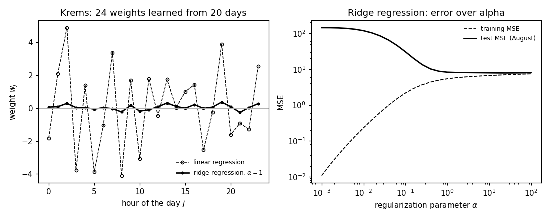
[B-figure]   The entry's figure: the 24 weights of the linear-regression
             and the ridge-regression hypothesis per hour, and the
             training and test MSE of ridge regression over a grid of
             alpha.

Outputs
-------
ridgeregression_krems.csv   : the data points, columns day,h0,...,h23,
                              next_tmax.
ridgeregression_weights.csv : columns hour,ls,ridge — the learned
                              weights per hour.
ridgeregression_alpha.csv   : columns alpha,train,test — MSE of ridge
                              regression over the alpha grid.
ridgeregression.png         : preview (checking only).
"""

# /// script
# requires-python = ">=3.10"
# dependencies = ["matplotlib==3.10.7", "numpy==2.3.4"]
# ///

import json
import urllib.request

import numpy as np
import matplotlib

matplotlib.use("Agg")
import matplotlib.pyplot as plt

from pathlib import Path

OUT_DIR = Path(__file__).parent

rng = np.random.default_rng(42)
report = []


def check(name, ok):
    report.append((name, bool(ok)))
    print(f"  [{'ok' if ok else 'FAIL'}] {name}")


def ridge(Xm, ym, alpha):
    """w_hat = (X^T X + alpha m I)^{-1} X^T y."""
    mm, dd = Xm.shape
    return np.linalg.solve(Xm.T @ Xm + alpha * mm * np.eye(dd), Xm.T @ ym)


def f_ridge(Xm, ym, alpha, w):
    """The penalized objective (1/m) ||y - X w||^2 + alpha ||w||^2."""
    return np.mean((ym - Xm @ w) ** 2) + alpha * w @ w


def mse(Xm, ym, w):
    return float(np.mean((Xm @ w - ym) ** 2))
Hourly air temperature (klima-v2-1h, tl) and daily maximum temperature (klima-v2-1d, tlmax) at Krems an der Donau, GeoSphere station 3805, July and August 2024. A data point is one day: feature vector x = its 24 hourly temperatures (d = 24), label y = the maximum temperature of the next day. Trainset: July 1 to 20 (m = 20 < d); test set: the 31 days of August.
BASE = "https://dataset.api.hub.geosphere.at/v1/station/historical/"


def fetch(query):
    with urllib.request.urlopen(BASE + query, timeout=120) as resp:
        return json.load(resp)


hourly = fetch("klima-v2-1h?parameters=tl&station_ids=3805"
               "&start=2024-07-01T00:00&end=2024-08-31T23:00")
daily = fetch("klima-v2-1d?parameters=tlmax&station_ids=3805"
              "&start=2024-07-01&end=2024-09-01")
tl = hourly["features"][0]["properties"]["parameters"]["tl"]["data"]
tmax = daily["features"][0]["properties"]["parameters"]["tlmax"]["data"]
days = [stamp[:10] for stamp in daily["timestamps"]]
check("[B-fetch] 62 days of 24 hourly temperatures and 63 daily maxima",
      len(tl) == 62 * 24 and len(tmax) == 63)
check("[B-fetch] no value is missing",
      all(t is not None for t in tl) and all(t is not None for t in tmax))
X_all = np.array(tl, dtype=float).reshape(62, 24)     # one row per day
y_all = np.array(tmax[1:], dtype=float)               # next day's maximum
with open(OUT_DIR / "ridgeregression_krems.csv", "w") as f:
    f.write("day," + ",".join(f"h{k}" for k in range(24)) + ",next_tmax\n")
    for day, row, lab in zip(days, X_all, y_all):
        f.write(day + "," + ",".join(f"{v:.1f}" for v in row) + f",{lab:.1f}\n")
m, d = 20, 24
X, y = X_all[:m], y_all[:m]                           # July 1 to 20
X_test, y_test = X_all[31:62], y_all[31:62]           # August 1 to 31
check("[B-fetch] trainset July 1-20 (m = 20 < d = 24), test set August (31 days)",
      X.shape == (20, 24) and days[0] == "2024-07-01" and days[19] == "2024-07-20"
      and X_test.shape == (31, 24) and days[31] == "2024-08-01")
  [ok] [B-fetch] 62 days of 24 hourly temperatures and 63 daily maxima
  [ok] [B-fetch] no value is missing
  [ok] [B-fetch] trainset July 1-20 (m = 20 < d = 24), test set August (31 days)
alpha = 1: the closed form zeroes the gradient of the penalized objective, the matrix X^T X + alpha m I is invertible although X^T X has rank 20 < 24, and random perturbations of w_hat increase the objective. Linear regression (the minimum-norm solution of the underdetermined normal equations, one of infinitely many) reproduces the training labels exactly (training MSE 0) and predicts August with MSE 141; ridge regression has training MSE 5.4 and test MSE 8.3.
ALPHA = 1.0
w_hat = ridge(X, y, ALPHA)
grad = -(2.0 / m) * X.T @ (y - X @ w_hat) + 2.0 * ALPHA * w_hat
check("[B-closed] the closed form satisfies the zero-gradient condition of the penalized objective",
      np.allclose(grad, 0.0))
check("[B-closed] random perturbations of w_hat increase the objective",
      all(f_ridge(X, y, ALPHA, w_hat + 0.1 * rng.normal(size=d))
          > f_ridge(X, y, ALPHA, w_hat) for _ in range(20)))
lam_min = np.linalg.eigvalsh(X.T @ X + ALPHA * m * np.eye(d)).min()
check("[B-closed] X^T X has rank 20 < 24, and X^T X + alpha m I is invertible "
      "(smallest eigenvalue >= alpha m)",
      np.linalg.matrix_rank(X.T @ X) == 20 and lam_min >= ALPHA * m - 1e-9)
w_ls = np.linalg.pinv(X) @ y                          # minimum-norm solution
null_dir = np.linalg.svd(X)[2][-1]                    # a null-space direction
check("[B-closed] the normal equations of linear regression are underdetermined: "
      "two different solutions reproduce the training labels",
      np.allclose(X @ w_ls, y) and np.allclose(X @ (w_ls + 5.0 * null_dir), y))
mse_ls_train, mse_ls_test = mse(X, y, w_ls), mse(X_test, y_test, w_ls)
mse_r_train, mse_r_test = mse(X, y, w_hat), mse(X_test, y_test, w_hat)
check(f"[B-closed] linear regression: training MSE {mse_ls_train:.1f}, "
      f"test MSE {mse_ls_test:.0f}",
      round(mse_ls_train, 1) == 0.0 and round(mse_ls_test) == 141)
check(f"[B-closed] ridge regression (alpha = 1): training MSE {mse_r_train:.1f}, "
      f"test MSE {mse_r_test:.1f}",
      round(mse_r_train, 1) == 5.4 and round(mse_r_test, 1) == 8.3)
  [ok] [B-closed] the closed form satisfies the zero-gradient condition of the penalized objective
  [ok] [B-closed] random perturbations of w_hat increase the objective
  [ok] [B-closed] X^T X has rank 20 < 24, and X^T X + alpha m I is invertible (smallest eigenvalue >= alpha m)
  [ok] [B-closed] the normal equations of linear regression are underdetermined: two different solutions reproduce the training labels
  [ok] [B-closed] linear regression: training MSE 0.0, test MSE 141
  [ok] [B-closed] ridge regression (alpha = 1): training MSE 5.4, test MSE 8.3
The singular values of X run from 504 down to 0.21; the hourly temperatures at 13:00 and 14:00 have correlation 0.93. The minimum-norm linear-regression solution is sum_j (v_j^T y / lambda_j) u_j; ridge multiplies each term by lambda_j^2 / (lambda_j^2 + alpha m), which lies strictly between 0 and 1; lambda_j / (lambda_j^2 + alpha m) never exceeds 1 / (2 sqrt(alpha m)) = 0.11, where 1 / lambda_j reaches 4.9; the four directions with lambda_j = 0 get weight 0. Label noise with variance 0.25 moves the linear-regression weights by 1.9 and the ridge weights by 0.2 (Euclidean norm). The condition number of X^T X + alpha m I is below that of X^T X restricted to its range.
Vf, sv, Ut = np.linalg.svd(X, full_matrices=False)   # X is 20 x 24, rank 20
corr_13_14 = float(np.corrcoef(X_all[:, 13], X_all[:, 14])[0, 1])
check(f"[B-svd] singular values from {sv[0]:.0f} down to {sv[-1]:.2f}; the "
      f"temperatures at 13:00 and 14:00 have correlation {corr_13_14:.2f}",
      round(sv[0]) == 504 and round(sv[-1], 2) == 0.21 and round(corr_13_14, 2) == 0.93)
coords = Vf.T @ y                                     # (v^(j))^T y
check("[B-svd] minimum-norm linear-regression solution = sum_j (v_j^T y / lambda_j) u_j",
      np.allclose(Ut.T @ (coords / sv), w_ls))
factor = sv ** 2 / (sv ** 2 + ALPHA * m)
check("[B-svd] ridge solution = shrinkage factor times each linear-regression term",
      np.allclose(Ut.T @ (factor * coords / sv), w_hat))
check("[B-svd] shrinkage factors lie strictly between 0 and 1",
      np.all((factor > 0.0) & (factor < 1.0)))
bound = 1.0 / (2.0 * np.sqrt(ALPHA * m))
amp_ridge, amp_ls = (sv / (sv ** 2 + ALPHA * m)).max(), (1.0 / sv).max()
check(f"[B-svd] lambda / (lambda^2 + alpha m) <= 1 / (2 sqrt(alpha m)) = {bound:.2f}, "
      f"where 1 / lambda reaches {amp_ls:.1f}",
      amp_ridge <= bound + 1e-12 and round(bound, 2) == 0.11 and round(amp_ls, 1) == 4.9)
U_all = np.linalg.svd(X)[2]                           # all 24 right singular vectors
check("[B-svd] ridge puts zero weight on the four directions with lambda_j = 0",
      np.allclose(U_all[20:] @ w_hat, 0.0))
noise = 0.5 * rng.normal(size=m)
move_ls = float(np.linalg.norm(np.linalg.pinv(X) @ (y + noise) - w_ls))
move_r = float(np.linalg.norm(ridge(X, y + noise, ALPHA) - w_hat))
check(f"[B-svd] label noise with variance 0.25 moves the linear-regression "
      f"weights by {move_ls:.1f} and the ridge weights by {move_r:.1f}",
      round(move_ls, 1) == 1.9 and round(move_r, 1) == 0.2)
cond_ridge = (sv[0] ** 2 + ALPHA * m) / (sv[-1] ** 2 + ALPHA * m)
cond_ls = sv[0] ** 2 / sv[-1] ** 2
check(f"[B-svd] condition number {cond_ridge:.0f} of X^T X + alpha m I is below "
      f"{cond_ls:.0f}, that of X^T X on its range", cond_ridge < cond_ls)
  [ok] [B-svd] singular values from 504 down to 0.21; the temperatures at 13:00 and 14:00 have correlation 0.93
  [ok] [B-svd] minimum-norm linear-regression solution = sum_j (v_j^T y / lambda_j) u_j
  [ok] [B-svd] ridge solution = shrinkage factor times each linear-regression term
  [ok] [B-svd] shrinkage factors lie strictly between 0 and 1
  [ok] [B-svd] lambda / (lambda^2 + alpha m) <= 1 / (2 sqrt(alpha m)) = 0.11, where 1 / lambda reaches 4.9
  [ok] [B-svd] ridge puts zero weight on the four directions with lambda_j = 0
  [ok] [B-svd] label noise with variance 0.25 moves the linear-regression weights by 1.9 and the ridge weights by 0.2
  [ok] [B-svd] condition number 12669 of X^T X + alpha m I is below 6038115, that of X^T X on its range
Augmentation equivalence (Bishop 1995): the average squared error loss over feature perturbations N(x, alpha I) equals the original loss plus exactly alpha ||w||^2 (Monte Carlo), and linear regression on a large augmented trainset recovers the ridge solution.
n_mc = 200_000
w_probe = rng.normal(size=d)
r = 0
eps = np.sqrt(ALPHA) * rng.normal(size=(n_mc, d))
loss_orig = (y[r] - X[r] @ w_probe) ** 2
loss_pert = np.mean((y[r] - (X[r] + eps) @ w_probe) ** 2)
excess = float(ALPHA * w_probe @ w_probe)
std_err = np.sqrt(2.0 * excess ** 2 + 4.0 * loss_orig * excess) / np.sqrt(n_mc)
check("[B-aug] average loss over perturbed copies = original loss + alpha ||w||^2 "
      "within four standard errors (Monte Carlo)",
      abs(loss_pert - loss_orig - excess) < 4.0 * std_err)
n_fit = 3000
X_aug = np.repeat(X, n_fit, axis=0) + np.sqrt(ALPHA) * rng.normal(size=(m * n_fit, d))
y_aug = np.repeat(y, n_fit)                           # labels left unchanged
w_aug = np.linalg.lstsq(X_aug, y_aug, rcond=None)[0]
check("[B-aug] linear regression on the augmented trainset recovers the ridge solution",
      np.allclose(w_aug, w_hat, atol=5e-2))
  [ok] [B-aug] average loss over perturbed copies = original loss + alpha ||w||^2 within four standard errors (Monte Carlo)
  [ok] [B-aug] linear regression on the augmented trainset recovers the ridge solution
The entry's figure: the 24 weights of the linear-regression and the ridge-regression hypothesis per hour, and the training and test MSE of ridge regression over a grid of alpha.
with open(OUT_DIR / "ridgeregression_weights.csv", "w") as f:
    f.write("hour,ls,ridge\n")
    for k in range(d):
        f.write(f"{k},{w_ls[k]:.3f},{w_hat[k]:.3f}\n")
alphas = np.logspace(-3, 2, 26)
curve = [(a, mse(X, y, ridge(X, y, a)), mse(X_test, y_test, ridge(X, y, a)))
         for a in alphas]
with open(OUT_DIR / "ridgeregression_alpha.csv", "w") as f:
    f.write("alpha,train,test\n")
    for a, tr, te in curve:
        f.write(f"{a:.5g},{tr:.3f},{te:.3f}\n")
best = min(curve, key=lambda c: c[2])
check(f"[B-figure] weights and the alpha grid written; test MSE is smallest at "
      f"alpha = {best[0]:.3g} ({best[2]:.1f})",
      len(curve) == 26 and w_ls.max() > 4.0 and abs(w_hat).max() < 0.5)

# ---- preview (checking only)
fig, (ax1, ax2) = plt.subplots(1, 2, figsize=(10, 4))
hours = np.arange(d)
ax1.plot(hours, w_ls, "k--o", lw=1, ms=4, mfc="none", label="linear regression")
ax1.plot(hours, w_hat, "k-", lw=1.8, marker=".", label=r"ridge regression, $\alpha = 1$")
ax1.axhline(0.0, color="0.7", lw=0.8)
ax1.set_xlabel("hour of the day $j$")
ax1.set_ylabel("weight $w_j$")
ax1.set_title("Krems: 24 weights learned from 20 days")
ax1.legend(frameon=False, fontsize=8)
ax2.loglog(alphas, [c[1] for c in curve], "k--", lw=1.2, label="training MSE")
ax2.loglog(alphas, [c[2] for c in curve], "k-", lw=1.8, label="test MSE (August)")
ax2.set_xlabel(r"regularization parameter $\alpha$")
ax2.set_ylabel("MSE")
ax2.set_title("Ridge regression: error over alpha")
ax2.legend(frameon=False, fontsize=8)
fig.tight_layout()
fig.savefig(OUT_DIR / "ridgeregression.png", dpi=110)

n_ok = sum(ok for _, ok in report)
print(f"\n{n_ok}/{len(report)} checks pass")
if n_ok != len(report):
    raise SystemExit(1)
  [ok] [B-figure] weights and the alpha grid written; test MSE is smallest at alpha = 25.1 (7.8)

20/20 checks pass
B-figure writes when the script runs