pythondemos/kernelridgeregression.pyDictionary of Applied Machine Learning
Updated on 2026-09-19
Typeset PDF version — the authoritative form of this entry
Python demo — a script that recomputes what this entry states and prints one line per check
Kernel ridge regression is a kernel method for regression that applies ridge regression to transformed feature vectors constructed from a kernel, and thereby learns a nonlinear hypothesis in closed form. It performs regularized empirical risk minimization (RERM) over the reproducing kernel Hilbert space (RKHS) of the kernel, combining the squared error loss with a squared-norm penalty term. By the representer theorem, the learned hypothesis is a weighted sum of kernel evaluations at the feature vectors in the training set, and the coefficients are obtained in closed form by solving a single system of linear equations. Like ridge regression, the method equals empirical risk minimization (ERM) on an augmented training set: the transformed feature vectors are perturbed by realizations of a zero-mean Gaussian process (GP) whose covariance function is the kernel scaled by the regularization parameter. For the kernel that is a modified inner product of the feature space, kernel ridge regression is ridge regression with a matching penalty term, and the perturbed copies of a data point fill an ellipse whose shape the kernel sets, the circle of ridge regression for the standard inner product.
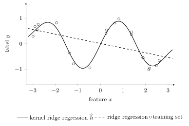
Consider a regression problem where the goal is to learn a hypothesis for predicting the numeric label of a data point based on its feature vector, but where the relation between features and label is nonlinear. An example is the prediction of the temperature over the course of a day from the time of the day, a relation that rises and falls over the day. Kernel ridge regression solves such regression problems by applying ridge regression to transformed feature vectors constructed from a kernel, and thereby learns a nonlinear hypothesis in closed form (Hastie et al., 2009, Sect. 5.8.2; Schölkopf and Smola, 2002). Fig. 1 shows a training set with a periodic relation between feature and label. With the Gaussian kernel $\kernelmap{\feature}{\feature'} = \exp\big( - (\feature - \feature')^{2} / (2 \sigma^{2}) \big)$ of bandwidth $\sigma = 0.7$, the learned hypothesis follows the data points smoothly, with a training mean squared error (MSE) of $0.013$, while ridge regression on the raw feature can only fit a straight line, with a training MSE of $0.36$.
B-dataFormally, kernel ridge regression learns a hypothesis from the reproducing kernel Hilbert space (RKHS) $\hilbertspace_{\kernel}$ of a kernel $\kernel: \featurespace \times \featurespace \rightarrow \reals$ by minimizing the penalized average squared error loss on a training set $\trainset = \big\{ \pair{\featurevec^{(\sampleidx)}}{\truelabel^{(\sampleidx)}} \big\}_{\sampleidx=1}^{\samplesize}$ with numeric labels $\truelabel^{(\sampleidx)} \in \reals$, \begin{equation} \label{eq:krr_rerm} \widehat{\hypothesis} = \argmin_{\hypothesis \in \hilbertspace_{\kernel}} \frac{1}{\samplesize} \sum_{\sampleidx=1}^{\samplesize} \big( \truelabel^{(\sampleidx)} - \hypothesis\big(\featurevec^{(\sampleidx)}\big) \big)^{2} + \regparam \normgeneric{\hypothesis}{\hilbertspace_{\kernel}}^{2} \text{.} \end{equation} The penalty term is the scaled squared RKHS norm $\regparam \normgeneric{\hypothesis}{\hilbertspace_{\kernel}}^{2}$ with a regularization parameter $\regparam > 0$. The resulting method is an instance of regularized empirical risk minimization (RERM), as is ridge regression, whose penalty term is the scaled squared Euclidean norm $\regparam \normgeneric{\weights}{2}^{2}$ of the model parameters (Hastie et al., 2009, Sect. 5.8.2). The average squared error loss is a convex function of $\hypothesis$, and the squared norm is strictly convex. The kernel ridge regression problem \(\eqref{eq:krr_rerm}\) therefore has a unique minimizer $\widehat{\hypothesis}$ for any training set, as does ridge regression.
B-closedBy the representer theorem (see kernel method), the minimizer
of the kernel ridge regression problem \(\eqref{eq:krr_rerm}\) has the
form
$\widehat{\hypothesis} = \sum_{\sampleidx=1}^{\samplesize} \expcoeff_{\sampleidx} \kernelmap{\featurevec^{(\sampleidx)}}{\cdot}$
with a coefficient vector
$\boldsymbol{\expcoeff} = \big(\expcoeff_{1}, \ldots, \expcoeff_{\samplesize}\big)^{\top}$.
Inserting this form into the kernel ridge regression problem
\(\eqref{eq:krr_rerm}\) yields the finite-dimensional optimization problem
\[
\min_{\boldsymbol{\expcoeff} \in \reals^{\samplesize}}
\frac{1}{\samplesize}
\normgeneric{\labelvec - \mK \boldsymbol{\expcoeff}}{2}^{2}
+ \regparam\, \boldsymbol{\expcoeff}^{\top} \mK \boldsymbol{\expcoeff}
\text{,}
\]
with the label vector
$\labelvec = \big(\truelabel^{(1)}, \ldots, \truelabel^{(\samplesize)}\big)^{\top}$
and the Gram matrix $\mK$ with entries
$K_{\sampleidx,\sampleidx'} = \kernelmap{\featurevec^{(\sampleidx)}}{\featurevec^{(\sampleidx')}}$
(see kernel). By the zero-gradient condition, a
coefficient vector solving this optimization problem satisfies
the system of linear equations
\[
\mK\big( \big(\mK + \regparam \samplesize \mI\big) \boldsymbol{\expcoeff} - \labelvec \big) = \mathbf{0} \text{.}
\]
Since $\mK$ is positive semi-definite (psd) and $\regparam > 0$, the matrix
$\mK + \regparam \samplesize \mI$ is invertible, and a
minimizer is obtained in closed form as
\begin{equation}
\label{eq:krr_closedform}
\widehat{\boldsymbol{\expcoeff}}
= \big( \mK + \regparam \samplesize \mI \big)^{-1} \labelvec
\text{.}
\end{equation}
The prediction for a data point with feature vector
$\featurevec$ is
\[
\widehat{\hypothesis}(\featurevec) = \sum_{\sampleidx=1}^{\samplesize} \widehat{\expcoeff}_{\sampleidx} \kernelmap{\featurevec^{(\sampleidx)}}{\featurevec} \text{.}
\]
Training is a one-shot computation: kernel ridge regression
requires no iterative optimization method (and hence no fixed-point
interpretation), only the unique solution of the
$\samplesize \times \samplesize$ system of linear equations
with the invertible matrix $\mK + \regparam \samplesize \mI$,
which is the closed form \(\eqref{eq:krr_closedform}\).
pythondemos/kernelridgeregression.py
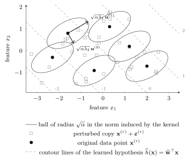
B-linkerLike ridge regression, kernel ridge regression has an interpretation as a form of data augmentation: training with noise added to the feature vectors is equivalent to adding a penalty term (Bishop, 1995), and replacing each data point by a probability distribution centered at it is the vicinal form of empirical risk minimization (ERM) (Chapelle et al., 2001), whose effect on kernel methods is a regularization of the learned hypothesis (Dao et al., 2019). Consider data points with two features, the feature space $\featurespace = \reals^{2}$, and the kernel \begin{equation} \label{eq:krr_metric_kernel} \kernelmap{\featurevec}{\featurevec'} \defeq \featurevec^{\top} \covmtxgeneric^{-1} \featurevec' \text{,} \end{equation} with a positive definite (pd) matrix $\covmtxgeneric \in \reals^{2 \times 2}$. This kernel is an inner product of $\reals^{2}$ with a modified metric: the squared norm $\kernelmap{\featurevec}{\featurevec} = \featurevec^{\top} \covmtxgeneric^{-1} \featurevec$ scales the two features differently and couples them, and its unit ball is an ellipse instead of the circle of the Euclidean norm. The RKHS $\hilbertspace_{\kernel}$ of this kernel is $\reals^{2}$ with this inner product. The transformed feature vector $\kernelmap{\featurevec}{\cdot}$ is the linear function $\featurevec' \mapsto \featurevec^{\top} \covmtxgeneric^{-1} \featurevec'$, every hypothesis in $\hilbertspace_{\kernel}$ is a linear model $\hypothesis^{(\weights)}(\featurevec) = \weights^{\top} \featurevec$ with model parameters $\weights \in \reals^{2}$, and its RKHS norm is $\normgeneric{\hypothesis^{(\weights)}}{\hilbertspace_{\kernel}}^{2} = \weights^{\top} \covmtxgeneric \weights$. The kernel ridge regression problem \(\eqref{eq:krr_rerm}\) therefore reads \begin{equation} \label{eq:krr_metric_ridge} \widehat{\weights} = \argmin_{\weights \in \reals^{2}} \frac{1}{\samplesize} \sum_{\sampleidx=1}^{\samplesize} \big( \truelabel^{(\sampleidx)} - \weights^{\top} \featurevec^{(\sampleidx)} \big)^{2} + \regparam \, \weights^{\top} \covmtxgeneric \weights \text{,} \end{equation} which is ridge regression with the penalty term $\regparam \normgeneric{\weights}{2}^{2}$ replaced by $\regparam \, \weights^{\top} \covmtxgeneric \weights$. Its unique minimizer is $\widehat{\weights} = \big( \featuremtx^{\top} \featuremtx + \regparam \samplesize \covmtxgeneric \big)^{-1} \featuremtx^{\top} \labelvec$ with the feature matrix $\featuremtx = \big(\featurevec^{(1)}, \ldots, \featurevec^{(\samplesize)}\big)^{\top}$, and it coincides with $\covmtxgeneric^{-1} \featuremtx^{\top} \widehat{\boldsymbol{\expcoeff}}$ for the coefficients \(\eqref{eq:krr_closedform}\) with the Gram matrix $\mK = \featuremtx \covmtxgeneric^{-1} \featuremtx^{\top}$. For $\covmtxgeneric = \mI$, the kernel \(\eqref{eq:krr_metric_kernel}\) is the linear kernel and the penalized problem \(\eqref{eq:krr_metric_ridge}\) is ridge regression itself.
B-metricAdding the penalty term in the penalized problem \(\eqref{eq:krr_metric_ridge}\) is equivalent to ERM on an augmented training set, i.e., to computing the average squared error loss of $\hypothesis^{(\weights)}$ on it. This augmented training set is obtained from the original training set. For each data point $\pair{\featurevec^{(\sampleidx)}}{\truelabel^{(\sampleidx)}}$, $\sampleidx = 1, \ldots, \samplesize$, the feature vector $\featurevec^{(\sampleidx)}$ is replaced by realizations of infinitely many independent and identically distributed (i.i.d.) random variables (RVs) $\featurevec^{(\sampleidx)} + \perturbation{\sampleidx}$ with Gaussian random variables (Gaussian RVs) $\perturbation{\sampleidx} \sim \mvnormal{\mathbf{0}}{\regparam \covmtxgeneric}$. The label $\truelabel^{(\sampleidx)}$ is left unchanged. The penalty term is exactly the amount by which the average squared error loss of $\hypothesis^{(\weights)}$ over the perturbed copies exceeds its squared error loss on the original data point. Since $\E \{ \perturbation{\sampleidx} \} = \mathbf{0}$, the increase is \[ \E \big\{ \big( \weights^{\top} \perturbation{\sampleidx} \big)^{2} \big\} = \weights^{\top} \E \big\{ \perturbation{\sampleidx} \big(\perturbation{\sampleidx}\big)^{\top} \big\} \weights = \regparam \, \weights^{\top} \covmtxgeneric \weights \text{.} \] The equivalence is exact for the linear model $\hypothesis^{(\weights)}$, while for a nonlinear hypothesis it holds up to terms of higher order in the noise amplitude (Bishop, 1995). As in ridge regression, this increase of the average loss under data augmentation is an estimate for the generalization gap. Accordingly, linear regression on a large augmented training set recovers the predictions of kernel ridge regression.
B-figureThe kernel determines the shape of these perturbations (see
Fig. 2). The covariance matrix
$\regparam \covmtxgeneric$ of $\perturbation{\sampleidx}$ is the
scaled inverse of the matrix in the kernel
\(\eqref{eq:krr_metric_kernel}\), so the one-standard-deviation
contour of the perturbed copies,
\[
\big(\featurevec - \featurevec^{(\sampleidx)}\big)^{\top} \covmtxgeneric^{-1} \big(\featurevec - \featurevec^{(\sampleidx)}\big) = \regparam \text{,}
\]
is the set of feature vectors $\featurevec$ with
$\kernelmap{\featurevec - \featurevec^{(\sampleidx)}}{\featurevec - \featurevec^{(\sampleidx)}} = \regparam$,
i.e., the ball of radius $\sqrt{\regparam}$ around
$\featurevec^{(\sampleidx)}$ in the norm induced by the
kernel. For $\covmtxgeneric = \mI$, this ball is a circle of
radius $\sqrt{\regparam}$: the perturbations in the data augmentation
interpretation of ridge regression have covariance matrix
$\regparam \mI$ and no preferred direction. For a general
$\covmtxgeneric$ it is an
ellipse, so the ellipses drawn around the data points display
the kernel: the size of a perturbation is measured by its
kernel norm, and the penalty term
$\regparam \, \weights^{\top} \covmtxgeneric \weights$ is the
average squared error loss that perturbations of kernel
norm $\sqrt{\regparam}$ cause. The ellipses also display
the matrix $\covmtxgeneric$ itself. Its eigenvalue decomposition (EVD)
$\covmtxgeneric = \sum_{\featureidx=1}^{2} \eigval{\featureidx} \eigvecCov^{(\featureidx)} \big(\eigvecCov^{(\featureidx)}\big)^{\top}$,
with eigenvalues $\eigval{1} \geq \eigval{2} > 0$ and
orthonormal eigenvectors $\eigvecCov^{(1)}, \eigvecCov^{(2)}$,
turns the contour into
\[
\sum_{\featureidx=1}^{2} \frac{\big( \big(\eigvecCov^{(\featureidx)}\big)^{\top} \big(\featurevec - \featurevec^{(\sampleidx)}\big) \big)^{2}}{\regparam \eigval{\featureidx}} = 1 \text{,}
\]
so the principal axes of every ellipse point along the
eigenvectors of $\covmtxgeneric$ and the semi-axes have
lengths $\sqrt{\regparam \eigval{1}}$ and
$\sqrt{\regparam \eigval{2}}$: the perturbations spread most
along the eigenvector with the largest eigenvalue, and
the penalty term charges a displacement along
$\eigvecCov^{(\featureidx)}$ at the rate $\eigval{\featureidx}$.
pythondemos/kernelridgeregression.py
See also: kernel method, ridge regression, kernel, reproducing kernel Hilbert space, regularized empirical risk minimization, squared error loss, regression, Gaussian process, data augmentation, feature transformation, penalty term.
@misc{dictml_kernelridgeregression,
  author = {Jung, Alexander and Olioumtsevits, Konstantina and Schnoor, Ekkehard},
  title = {kernel ridge regression},
  howpublished = {Dictionary of Applied Machine Learning (course edition)},
  year = {2026},
  doi = {10.5281/zenodo.21569296},
  note = {ISBN 978-952-64-3013-3, CC BY 4.0, retrieved 2026-09-21},
  url = {https://dictionaryofml.org/terms/kernelridgeregression.html}
}