B-figure writes when the script runsDictionary of Applied Machine Learning · kernel ridge regression
Numerical companion to the entry kernel ridge regression: it recomputes what the entry states and prints one line per check
Kernel ridge regression (KRR) is RERM over the RKHS H_k with the squared error loss,
Run it with python3 kernelridgeregression.py, from any directory — it writes its output files into the current directory. Requires NumPy and Matplotlib only, and uses fixed seeds, so the printed numbers reproduce exactly. Download kernelridgeregression.py · Notebook · Open in Colab
One cell per block of the script: the code, and what that code printed when it last ran here
"""
kernelridgeregression.py — numerical companion to the glossary entry
'kernel ridge regression'.

Purpose
-------
Kernel ridge regression (KRR) is RERM over the RKHS H_k with the squared
error loss,

    min_{h in H_k}  (1/m) sum_r (y^(r) - h(x^(r)))^2  +  alpha ||h||_{H_k}^2 ,

whose representer-theorem solution h_hat = sum_r beta_r k(x^(r), .) has the
closed-form expansion coefficients  beta_hat = (K + alpha m I)^{-1} y  with
Gram matrix K_rs = k(x^(r), x^(s)).  The demo verifies the closed form on a
one-dimensional trainset, the reduction to ridge regression for the linear
kernel, and the data augmentation interpretation (Bishop 1995) in the
setting of the entry: the kernel k(x, x') = x^T C^{-1} x' on two features,
whose RKHS is R^2 with the modified inner product, so that KRR is ridge
regression with the penalty alpha w^T C w and the augmentation perturbs the
raw feature vectors with covariance alpha C, i.e., within the ellipse of
radius sqrt(alpha) in the norm induced by the kernel.  Self-contained
(numpy/matplotlib only), fixed seeds.

Blocks
------
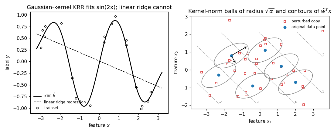
[B-data]     m = 20 scalar features x^(r) uniform in [-3, 3] (seed 0),
             labels y^(r) = sin(2 x^(r)) + 0.15 * noise.
[B-closed]   Gaussian kernel (sigma = 0.7), alpha = 1e-2: closed-form
             beta_hat solves (K + alpha m I) beta = y up to rounding
             error; training MSE below the noise level; linear ridge
             regression on [x, 1] with the same alpha fits a straight
             line with a training MSE more than ten times larger.
[B-linker]   Linear kernel k(x, x') = x^T x' on a two-feature trainset:
             KRR predictions coincide with ridge regression on the raw
             feature vectors (same alpha).
[B-metric]   Kernel k(x, x') = x^T C^{-1} x' with C = R diag(1.5^2, 0.75^2)
             R^T, R the rotation by 30 degrees (eigenvalues 1.5^2, 0.75^2,
             eigenvectors at 30 degrees to the feature axes):
             the KRR prediction sum_r beta_r k(x^(r), x) equals w_hat^T x
             with w_hat = (X^T X + alpha m C)^{-1} X^T y = C^{-1} X^T
             beta_hat (ridge regression with penalty alpha w^T C w); the
             average squared error loss over perturbed copies x^(r) +
             eps, eps ~ N(0, alpha C), exceeds the original loss by
             exactly alpha w^T C w (Monte Carlo); linear regression on a
             large augmented trainset recovers w_hat; the random function
             k(eps, .) has covariance alpha k(x, x') (Monte Carlo, four
             standard errors); on the ellipse (x - x^(r))^T C^{-1}
             (x - x^(r)) = alpha the kernel norm of the perturbation is
             sqrt(alpha).
[B-figure]   Two-feature trainset of six data points for the entry's
             augmentation figure (alpha = 1/2): the one-standard-deviation
             ellipse of the perturbation around each data point, i.e.,
             the ball of radius sqrt(alpha) in the kernel norm, six
             perturbed copies per point, and the contour lines w_hat^T x
             = c of the hypothesis learned from the six labelled points
             (closed form with the figure's alpha and C), clipped to the
             axis box, with their level values; on one ellipse the two
             principal axes sqrt(alpha lambda_j) u^(j), the eigenvectors
             u^(j) of C scaled by the square roots of alpha times its
             eigenvalues lambda_j, which end on the ellipse.

Outputs
-------
kernelridgeregression_points.csv       : the 1-D trainset, columns x,y.
kernelridgeregression_curves.csv       : dense grid, columns x,krr,lin
                                         (KRR fit and linear-ridge fit).
kernelridgeregression_aug_points.csv   : the six original feature
                                         vectors, columns x1,x2.
kernelridgeregression_aug_copies.csv   : the perturbed copies, x1,x2.
kernelridgeregression_aug_ellipses.csv : the six ellipses as polylines
                                         separated by nan rows, x1,x2.
kernelridgeregression_aug_contours.csv : contour lines of w_hat^T x as
                                         segments separated by nan rows.
kernelridgeregression_aug_labels.csv   : x1,x2,label — the right-hand end
                                         of each contour line and its level.
kernelridgeregression_aug_axis1.csv,
kernelridgeregression_aug_axis2.csv    : the two principal axes of one
                                         ellipse, center and tip, x1,x2.
kernelridgeregression.png              : preview (checking only).
"""

import numpy as np
import matplotlib

matplotlib.use("Agg")
import matplotlib.pyplot as plt

from pathlib import Path

OUT_DIR = Path(__file__).parent

report = []


def check(name, ok):
    report.append((name, bool(ok)))
    print(f"  [{'ok' if ok else 'FAIL'}] {name}")


def krr_coefficients(K, y, alpha):
    """beta_hat = (K + alpha m I)^{-1} y."""
    m = len(y)
    return np.linalg.solve(K + alpha * m * np.eye(m), y)


def ridge(Xm, ym, alpha):
    """w_hat = (X^T X + alpha m I)^{-1} X^T y (the ridgeregression entry)."""
    mm, dd = Xm.shape
    return np.linalg.solve(Xm.T @ Xm + alpha * mm * np.eye(dd), Xm.T @ ym)
m = 20 scalar features x^(r) uniform in [-3, 3] (seed 0), labels y^(r) = sin(2 x^(r)) + 0.15 * noise.
rng = np.random.default_rng(0)
m = 20
x = np.sort(rng.uniform(-3.0, 3.0, m))
y = np.sin(2.0 * x) + 0.15 * rng.standard_normal(m)
check("[B-data] m = 20 noisy samples of sin(2x)", m == 20)
[ok] [B-data] m = 20 noisy samples of sin(2x)
Gaussian kernel (sigma = 0.7), alpha = 1e-2: closed-form beta_hat solves (K + alpha m I) beta = y up to rounding error; training MSE below the noise level; linear ridge regression on [x, 1] with the same alpha fits a straight line with a training MSE more than ten times larger.
SIGMA = 0.7
ALPHA = 1e-2


def gauss_kernel_1d(p, q):
    return np.exp(-(p[:, None] - q[None, :]) ** 2 / (2.0 * SIGMA ** 2))


K = gauss_kernel_1d(x, x)
beta = krr_coefficients(K, y, ALPHA)


def h_hat(p):
    """Representer expansion: h_hat(x) = sum_r beta_r k(x^(r), x)."""
    return gauss_kernel_1d(p, x) @ beta


residual = float(np.linalg.norm((K + ALPHA * m * np.eye(m)) @ beta - y))
mse_krr = float(np.mean((h_hat(x) - y) ** 2))
X1 = np.c_[x, np.ones(m)]
w_lin = ridge(X1, y, ALPHA)
mse_lin = float(np.mean((X1 @ w_lin - y) ** 2))
check("[B-closed] beta_hat solves (K + alpha m I) beta = y", residual < 1e-10)
check(f"[B-closed] KRR training MSE {mse_krr:.4f} < 0.05", mse_krr < 0.05)
check(f"[B-closed] linear ridge MSE {mse_lin:.3f} > 10 x KRR MSE",
      mse_lin > 10.0 * mse_krr)

grid = np.linspace(-3.2, 3.2, 201)
with open(OUT_DIR / "kernelridgeregression_points.csv", "w") as f:
    f.write("x,y\n")
    for xi, yi in zip(x, y):
        f.write(f"{xi:.4f},{yi:.4f}\n")
with open(OUT_DIR / "kernelridgeregression_curves.csv", "w") as f:
    f.write("x,krr,lin\n")
    for g, a, b in zip(grid, h_hat(grid), np.c_[grid, np.ones_like(grid)] @ w_lin):
        f.write(f"{g:.4f},{a:.4f},{b:.4f}\n")
  [ok] [B-closed] beta_hat solves (K + alpha m I) beta = y
  [ok] [B-closed] KRR training MSE 0.0129 < 0.05
  [ok] [B-closed] linear ridge MSE 0.363 > 10 x KRR MSE
Linear kernel k(x, x') = x^T x' on a two-feature trainset: KRR predictions coincide with ridge regression on the raw feature vectors (same alpha).
rng2 = np.random.default_rng(1)
m2 = 30
X2 = rng2.normal(size=(m2, 2))
y2 = X2 @ np.array([1.5, -0.7]) + 0.2 * rng2.normal(size=m2)
X2_new = rng2.normal(size=(50, 2))
beta_lin = krr_coefficients(X2 @ X2.T, y2, ALPHA)
pred_krr = X2_new @ X2.T @ beta_lin          # sum_r beta_r x^(r)^T x
pred_ridge = X2_new @ ridge(X2, y2, ALPHA)
check("[B-linker] linear-kernel KRR predictions equal ridge regression on "
      "the raw feature vectors", np.allclose(pred_krr, pred_ridge))
[ok] [B-linker] linear-kernel KRR predictions equal ridge regression on the raw feature vectors
Kernel k(x, x') = x^T C^{-1} x' with C = R diag(1.5^2, 0.75^2) R^T, R the rotation by 30 degrees (eigenvalues 1.5^2, 0.75^2, eigenvectors at 30 degrees to the feature axes): the KRR prediction sum_r beta_r k(x^(r), x) equals w_hat^T x with w_hat = (X^T X + alpha m C)^{-1} X^T y = C^{-1} X^T beta_hat (ridge regression with penalty alpha w^T C w); the average squared error loss over perturbed copies x^(r) + eps, eps ~ N(0, alpha C), exceeds the original loss by exactly alpha w^T C w (Monte Carlo); linear regression on a large augmented trainset recovers w_hat; the random function k(eps, .) has covariance alpha k(x, x') (Monte Carlo, four standard errors); on the ellipse (x - x^(r))^T C^{-1} (x - x^(r)) = alpha the kernel norm of the perturbation is sqrt(alpha).
THETA_C = np.pi / 6                                 # principal axes at 30 degrees
R_C = np.array([[np.cos(THETA_C), -np.sin(THETA_C)],
                [np.sin(THETA_C), np.cos(THETA_C)]])
EIGVALS_C = np.array([1.5 ** 2, 0.75 ** 2])
C = R_C @ np.diag(EIGVALS_C) @ R_C.T               # pd, eigenvectors = columns of R_C
C_inv = np.linalg.inv(C)


def metric_kernel(P, Q):
    return P @ C_inv @ Q.T


beta_m = krr_coefficients(metric_kernel(X2, X2), y2, ALPHA)
w_metric = np.linalg.solve(X2.T @ X2 + ALPHA * m2 * C, X2.T @ y2)
check("[B-metric] w_hat = (X^T X + alpha m C)^{-1} X^T y equals C^{-1} X^T beta_hat",
      np.allclose(w_metric, C_inv @ X2.T @ beta_m))
check("[B-metric] KRR predictions equal w_hat^T x (ridge regression with "
      "penalty alpha w^T C w)",
      np.allclose(metric_kernel(X2_new, X2) @ beta_m, X2_new @ w_metric))

w_probe = rng2.normal(size=2)
r = 0
n_mc = 200_000
eps = rng2.multivariate_normal(np.zeros(2), ALPHA * C, size=n_mc)
loss_orig = (y2[r] - X2[r] @ w_probe) ** 2
loss_pert = np.mean((y2[r] - (X2[r] + eps) @ w_probe) ** 2)
excess = float(ALPHA * w_probe @ C @ w_probe)     # variance of w^T eps
std_err = np.sqrt(2.0 * excess ** 2 + 4.0 * loss_orig * excess) / np.sqrt(n_mc)
print(f"  excess loss {loss_pert - loss_orig:.5f}, alpha w^T C w {excess:.5f}, "
      f"standard error {std_err:.5f}")
check("[B-metric] average loss over perturbed copies = original loss + "
      "alpha w^T C w within four standard errors (Monte Carlo)",
      abs(loss_pert - loss_orig - excess) < 4.0 * std_err)
n_fit = 3000
X_aug = np.repeat(X2, n_fit, axis=0) \
    + rng2.multivariate_normal(np.zeros(2), ALPHA * C, size=m2 * n_fit)
y_aug = np.repeat(y2, n_fit)                        # labels left unchanged
w_aug = np.linalg.lstsq(X_aug, y_aug, rcond=None)[0]
check("[B-metric] linear regression on the augmented trainset recovers w_hat",
      np.allclose(w_aug, w_metric, atol=5e-2))
# covariance of the random function k(eps, .)
pairs = rng2.normal(size=(4, 2, 2))
cov_ok = True
for xa, xb in pairs:
    ka, kb = eps @ C_inv @ xa, eps @ C_inv @ xb        # k(eps, xa), k(eps, xb)
    emp = np.mean(ka * kb)
    k_ab = float(xa @ C_inv @ xb)
    k_aa, k_bb = float(xa @ C_inv @ xa), float(xb @ C_inv @ xb)
    std_err = ALPHA * np.sqrt(k_ab ** 2 + k_aa * k_bb) / np.sqrt(n_mc)
    cov_ok &= abs(emp - ALPHA * k_ab) < 4.0 * std_err
check("[B-metric] E{k(eps, x) k(eps, x')} = alpha k(x, x') within four "
      "standard errors (Monte Carlo, 4 pairs)", bool(cov_ok))
theta = np.linspace(0, 2 * np.pi, 61)
L = np.linalg.cholesky(C)


def ellipse(alpha):
    """The contour d^T C^{-1} d = alpha, i.e., k(d, d) = alpha."""
    return np.sqrt(alpha) * (L @ np.stack([np.cos(theta), np.sin(theta)])).T


ring = ellipse(ALPHA)
check("[B-metric] on the one-standard-deviation ellipse the kernel norm of "
      "the perturbation is sqrt(alpha)",
      np.allclose(np.sqrt(np.einsum("ij,jk,ik->i", ring, C_inv, ring)),
                  np.sqrt(ALPHA)))
  [ok] [B-metric] w_hat = (X^T X + alpha m C)^{-1} X^T y equals C^{-1} X^T beta_hat
  [ok] [B-metric] KRR predictions equal w_hat^T x (ridge regression with penalty alpha w^T C w)
  excess loss 0.01008, alpha w^T C w 0.01043, standard error 0.00041
  [ok] [B-metric] average loss over perturbed copies = original loss + alpha w^T C w within four standard errors (Monte Carlo)
  [ok] [B-metric] linear regression on the augmented trainset recovers w_hat
  [ok] [B-metric] E{k(eps, x) k(eps, x')} = alpha k(x, x') within four standard errors (Monte Carlo, 4 pairs)
  [ok] [B-metric] on the one-standard-deviation ellipse the kernel norm of the perturbation is sqrt(alpha)
Two-feature trainset of six data points for the entry's augmentation figure (alpha = 1/2): the one-standard-deviation ellipse of the perturbation around each data point, i.e., the ball of radius sqrt(alpha) in the kernel norm, six perturbed copies per point, and the contour lines w_hat^T x = c of the hypothesis learned from the six labelled points (closed form with the figure's alpha and C), clipped to the axis box, with their level values; on one ellipse the two principal axes sqrt(alpha lambda_j) u^(j), the eigenvectors u^(j) of C scaled by the square roots of alpha times its eigenvalues lambda_j, which end on the ellipse.
ALPHA_FIG = 0.5
rng3 = np.random.default_rng(3)
P = np.array([[-1.6, 0.8], [-0.4, -0.9], [0.3, 1.1], [1.2, 0.2],
              [2.0, -0.7], [-2.3, -0.3]])
copies = np.vstack([p + rng3.multivariate_normal(np.zeros(2), ALPHA_FIG * C, size=6)
                    for p in P])
ring_fig = ellipse(ALPHA_FIG)
with open(OUT_DIR / "kernelridgeregression_aug_points.csv", "w") as f:
    f.write("x1,x2\n")
    for p in P:
        f.write(f"{p[0]:.3f},{p[1]:.3f}\n")
with open(OUT_DIR / "kernelridgeregression_aug_copies.csv", "w") as f:
    f.write("x1,x2\n")
    for c in copies:
        f.write(f"{c[0]:.3f},{c[1]:.3f}\n")
with open(OUT_DIR / "kernelridgeregression_aug_ellipses.csv", "w") as f:
    f.write("x1,x2\n")
    for p in P:
        for e in ring_fig + p:
            f.write(f"{e[0]:.3f},{e[1]:.3f}\n")
        f.write("nan,nan\n")
# labels for the six data points, the learned hypothesis, and its contour lines
y_fig = P @ np.array([0.8, 1.2]) + 0.3 * rng3.normal(size=len(P))
w_fig = np.linalg.solve(P.T @ P + ALPHA_FIG * len(P) * C, P.T @ y_fig)
beta_fig = krr_coefficients(metric_kernel(P, P), y_fig, ALPHA_FIG)
check("[B-figure] w_hat on the six data points equals C^{-1} X^T beta_hat",
      np.allclose(w_fig, C_inv @ P.T @ beta_fig))
BOX = (-3.5, 3.5, -1.9, 2.1)                       # the figure's axis limits


def clip_line(w, c, box):
    """Endpoints of the line w^T x = c inside the box (None if it misses)."""
    x1min, x1max, x2min, x2max = box
    pts = []
    for x1 in (x1min, x1max):                       # crossings of the sides
        if abs(w[1]) > 1e-12:
            x2 = (c - w[0] * x1) / w[1]
            if x2min - 1e-9 <= x2 <= x2max + 1e-9:
                pts.append((x1, x2))
    for x2 in (x2min, x2max):                       # crossings of top/bottom
        if abs(w[0]) > 1e-12:
            x1 = (c - w[1] * x2) / w[0]
            if x1min - 1e-9 <= x1 <= x1max + 1e-9:
                pts.append((x1, x2))
    pts = sorted(set((round(a, 6), round(b, 6)) for a, b in pts))
    return (pts[0], pts[-1]) if len(pts) >= 2 else None


corners = np.array([[BOX[0], BOX[2]], [BOX[0], BOX[3]], [BOX[1], BOX[2]], [BOX[1], BOX[3]]])
vals = corners @ w_fig
step = 1.0 if vals.max() - vals.min() < 6.0 else 2.0
levels = np.arange(np.ceil(vals.min()), np.floor(vals.max()) + 1e-9, step)
segments = [(c, clip_line(w_fig, c, BOX)) for c in levels]
segments = [(c, seg) for c, seg in segments if seg is not None]
with open(OUT_DIR / "kernelridgeregression_aug_contours.csv", "w") as f:
    f.write("x1,x2\n")
    for c, (p0, p1) in segments:
        f.write(f"{p0[0]:.3f},{p0[1]:.3f}\n{p1[0]:.3f},{p1[1]:.3f}\nnan,nan\n")
with open(OUT_DIR / "kernelridgeregression_aug_labels.csv", "w") as f:
    f.write("x1,x2,label\n")
    for c, (p0, p1) in segments:
        p = p1 if p1[0] >= p0[0] else p0            # the right-hand endpoint
        f.write(f"{p[0]:.3f},{p[1]:.3f},{c:g}\n")
print(f"  hypothesis on the figure's trainset: w_hat = ({w_fig[0]:.2f}, "
      f"{w_fig[1]:.2f}); contour levels {levels}")
# principal axes of the ellipse: eigenvectors of C, semi-axes sqrt(alpha lambda_j)
lam, U = np.linalg.eigh(C)
order = np.argsort(lam)[::-1]
lam, U = lam[order], U[:, order]
U = U * np.sign(U[0, :])                            # orient each axis rightwards
semi = np.sqrt(ALPHA_FIG * lam)
p_axes = P[0]                                       # the ellipse that carries the arrows
for jx in range(2):
    tip = p_axes + semi[jx] * U[:, jx]
    with open(OUT_DIR / f"kernelridgeregression_aug_axis{jx + 1}.csv", "w") as f:
        f.write("x1,x2\n")
        f.write(f"{p_axes[0]:.3f},{p_axes[1]:.3f}\n{tip[0]:.3f},{tip[1]:.3f}\n")
quad = [float((semi[jx] * U[:, jx]) @ C_inv @ (semi[jx] * U[:, jx])) for jx in range(2)]
check("[B-figure] the principal axes sqrt(alpha lambda_j) u^(j) of C end on "
      "the ellipse d^T C^{-1} d = alpha", np.allclose(quad, ALPHA_FIG))
check("[B-figure] the eigenvectors of C are the axes at 30 degrees",
      np.allclose(np.abs(U[:, 0] @ R_C[:, 0]), 1.0) and np.isclose(lam[0], EIGVALS_C[0]))
print(f"  principal axes on x^(1) = ({p_axes[0]:.2f}, {p_axes[1]:.2f}): tips "
      f"({(p_axes + semi[0] * U[:, 0])[0]:.2f}, {(p_axes + semi[0] * U[:, 0])[1]:.2f}) and "
      f"({(p_axes + semi[1] * U[:, 1])[0]:.2f}, {(p_axes + semi[1] * U[:, 1])[1]:.2f}); "
      f"semi-axes {semi[0]:.2f}, {semi[1]:.2f}")
check("[B-figure] six data points, 36 perturbed copies, six ellipses, "
      f"{len(segments)} contour lines written",
      len(P) == 6 and len(copies) == 36 and len(segments) >= 4)

# ---- preview (checking only)
fig, (ax1, ax2) = plt.subplots(1, 2, figsize=(10, 4))
ax1.plot(grid, h_hat(grid), "k-", lw=1.8, label="KRR $\\hat{h}$")
ax1.plot(grid, np.c_[grid, np.ones_like(grid)] @ w_lin, "k--", lw=1.2,
         label="linear ridge regression")
ax1.plot(x, y, "ko", ms=4, mfc="none", label="trainset")
ax1.set_xlabel("feature $x$")
ax1.set_ylabel("label $y$")
ax1.set_title("Gaussian-kernel KRR fits sin(2x); linear ridge cannot")
ax1.legend(frameon=False, fontsize=8)
for p in P:
    e = ring_fig + p
    ax2.plot(e[:, 0], e[:, 1], color="0.5", lw=1)
for jx in range(2):
    tip = p_axes + semi[jx] * U[:, jx]
    ax2.annotate("", xy=tip, xytext=p_axes, arrowprops=dict(arrowstyle="->", lw=1.2))
for c, (p0, p1) in segments:
    ax2.plot([p0[0], p1[0]], [p0[1], p1[1]], color="0.6", lw=0.8, ls="--")
    ax2.annotate(f"{c:g}", (p1 if p1[0] >= p0[0] else p0), fontsize=7,
                 color="0.4", ha="left", va="bottom")
ax2.scatter(copies[:, 0], copies[:, 1], marker="s", facecolors="none",
            edgecolors="tab:red", s=16, label="perturbed copy")
ax2.scatter(P[:, 0], P[:, 1], marker="o", color="tab:blue", s=30,
            label="original data point")
ax2.set_aspect("equal")
ax2.set_xlabel("feature $x_1$")
ax2.set_ylabel("feature $x_2$")
ax2.set_title("Kernel-norm balls of radius $\\sqrt{\\alpha}$ and contours of $\\hat{w}^T x$")
ax2.legend(frameon=False, fontsize=8)
fig.tight_layout()
fig.savefig(OUT_DIR / "kernelridgeregression.png", dpi=110)

n_ok = sum(ok for _, ok in report)
print(f"\n{n_ok}/{len(report)} checks pass")
if n_ok != len(report):
    raise SystemExit(1)
  [ok] [B-figure] w_hat on the six data points equals C^{-1} X^T beta_hat
  hypothesis on the figure's trainset: w_hat = (0.47, 0.48); contour levels [-2. -1.  0.  1.  2.]
  [ok] [B-figure] the principal axes sqrt(alpha lambda_j) u^(j) of C end on the ellipse d^T C^{-1} d = alpha
  [ok] [B-figure] the eigenvectors of C are the axes at 30 degrees
  principal axes on x^(1) = (-1.60, 0.80): tips (-0.68, 1.33) and (-1.33, 0.34); semi-axes 1.06, 0.53
  [ok] [B-figure] six data points, 36 perturbed copies, six ellipses, 5 contour lines written

15/15 checks pass
B-figure writes when the script runs