B-plot writes when the script runsDictionary of Applied Machine Learning · maximum likelihood
Updated on 2026-11-19
Numerical companion to the entry maximum likelihood: it recomputes what the entry states and prints one line per check
Numerical companion to the glossary entry 'maxlikelihood'. The 366 daily maximum temperatures of 2024 at Krems (GeoSphere station 3805) are modeled as realizations of i.i.d. Gaussian random variables with unknown mean and variance. Maximum likelihood chooses the two parameters under which the observed year has the largest probability density.
Run it without installing anything:uv run https://dictionaryofml.org/terms/maxlikelihood.py
uv downloads this script and the pinned NumPy and Matplotlib it needs, then runs it; the script fetches any input file it uses. To keep the output files, download maxlikelihood.py into a folder and run uv run maxlikelihood.py there. With NumPy and Matplotlib already installed, python3 maxlikelihood.py, from any directory — it writes its output files into the current directory. Fixed seeds, so the printed numbers reproduce exactly. Download maxlikelihood.py · Notebook · Open in Colab
Before running a downloaded copy, scan it: uvx bandit -q -t B102,B307,B602,B605 maxlikelihood.py (B102,B307,B602,B605 are the exec, eval and shell checks of bandit) reports nothing: the script runs no shell command and evaluates no generated code.
One cell per block of the script: the code, and what that code printed when it last ran here
"""Maximum likelihood for the daily maximum temperature at Krems an der
Donau: the Gaussian that makes one year of observations most probable.

Purpose
-------
Numerical companion to the glossary entry 'maxlikelihood'.  The 366 daily
maximum temperatures of 2024 at Krems (GeoSphere station 3805) are modeled
as realizations of i.i.d. Gaussian random variables with unknown mean and
variance.  Maximum likelihood chooses the two parameters under which the
observed year has the largest probability density.

The demo checks the entry's claims: the maximum likelihood estimates of a
Gaussian are the sample mean and the mean squared deviation (closed
forms, the zero-gradient condition of the log-likelihood); the average
log-likelihood as a function of the mean is a concave parabola whose
curvature is the negative Fisher information; the negative log-likelihood
per data point is the average of a loss, an affine function of the
average squared error, so maximum likelihood is ERM, the minimization
of a training error; the variance estimate is biased by the factor
(m-1)/m; enlarging the hypothesis space to one mean per calendar day lets the
likelihood grow without bound while the log-likelihood of the preceding
year falls without bound (overfitting), whereas twelve monthly means
improve both years.

Deterministic: no random numbers are drawn.  Self-contained: numpy +
matplotlib only; the GeoSphere download falls back to the committed CSV.

Blocks
------
[B-data]       Download the daily maximum temperature of 2023 and 2024 at
               Krems (GeoSphere station 3805) or read the committed copy;
               731 days, no missing value.
[B-closedform] The Gaussian with the largest likelihood on the 366 days
               of 2024: mean = sample mean, variance = mean squared
               deviation; the gradient of the log-likelihood vanishes
               there and no grid point does better; the variance
               estimate is (m-1)/m times the sum of squared deviations
               divided by m-1 (the unbiased estimate of the variance).
[B-loglik]     The average log-likelihood as a function of the mean, with
               the variance fixed at its estimate: a concave parabola
               with vertex at the sample mean and second derivative
               -1/variance, the negative Fisher information; the same
               curve for the 365 days of 2023 peaks at the 2023 mean.
[B-erm]        The negative log-likelihood per day is the average of a
               loss; for a fixed variance it is an affine function of the
               average squared error, so both have the same minimizer.
[B-hypospace]  Three hypothesis spaces: one Gaussian, twelve monthly
               means with a common variance, one mean per calendar day
               with a common variance.  Average log-likelihood of the
               training year 2024 and of the held-out year 2023: the
               monthly means improve both, the daily means drive the
               training value above every bound and the held-out value
               below every bound as the variance shrinks to zero.
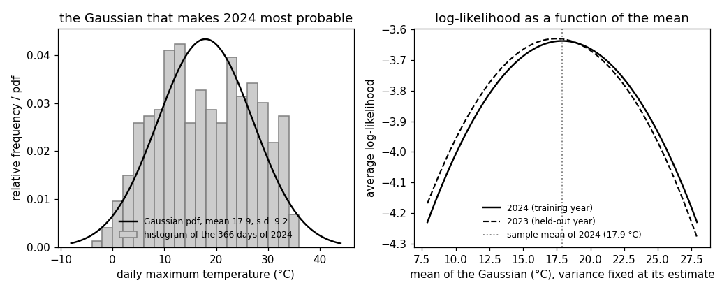
[B-plot]       Histogram and Gaussian pdf, the two log-likelihood
               curves, and the preview figure.

Outputs
-------
maxlikelihood_weather.csv : date, tmax for 2023 and 2024 (committed copy).
maxlikelihood_hist.csv    : t, freq -- histogram of the 2024 maxima,
                            bin edges (ybar interval), density scale.
maxlikelihood_pdf.csv     : t, pdf -- the maximum likelihood Gaussian.
maxlikelihood_loglik.csv  : mu, ll2024, ll2023 -- average log-likelihood
                            against the mean, variance fixed at the 2024
                            estimate.
maxlikelihood.png         : matplotlib preview (checking only).
"""

# /// script
# requires-python = ">=3.10"
# dependencies = ["matplotlib==3.10.7", "numpy==2.3.4"]
# ///

import json
import urllib.request
from pathlib import Path

import numpy as np
import matplotlib

matplotlib.use("Agg")
import matplotlib.pyplot as plt

OUT_DIR = Path(__file__).parent

report = []


def check(name, ok):
    report.append((name, bool(ok)))
    print(f"  [{'ok' if ok else 'FAIL'}] {name}")
Download the daily maximum temperature of 2023 and 2024 at Krems (GeoSphere station 3805) or read the committed copy; 731 days, no missing value.
print("[B-data] daily maximum temperature at Krems, 2023 and 2024")
URL = ("https://dataset.api.hub.geosphere.at/v1/station/historical/"
       "klima-v2-1d?parameters=tlmax&station_ids=3805"
       "&start=2023-01-01&end=2024-12-31")
CSV = OUT_DIR / "maxlikelihood_weather.csv"
try:
    with urllib.request.urlopen(URL, timeout=120) as resp:
        payload = json.load(resp)
    values = payload["features"][0]["properties"]["parameters"]["tlmax"]
    records = [(stamp[:10], hi)
               for stamp, hi in zip(payload["timestamps"], values["data"])]
    with open(CSV, "w") as fh:
        fh.write("date,tmax\n")
        for day, hi in records:
            fh.write(f"{day},{hi}\n")
    print(f"    downloaded {len(records)} days")
except OSError as err:
    print(f"    download failed ({err}); reading the committed CSV")
    rows = CSV.read_text().strip().splitlines()[1:]
    records = [(d, float(v)) for d, v in (r.split(",") for r in rows)]

check("[B-data] 731 days for 2023 and 2024", len(records) == 731)
check("[B-data] no day is missing its maximum temperature",
      all(hi is not None for _, hi in records))
dates = np.array([d for d, _ in records])
tmax = np.array([hi for _, hi in records], dtype=float)
is24 = np.array([d.startswith("2024") for d in dates])
x = tmax[is24]            # the training year: 366 realizations
x23 = tmax[~is24]         # the held-out year: 365 realizations
m = len(x)
check(f"[B-data] {m} days in 2024 and {len(x23)} days in 2023",
      m == 366 and len(x23) == 365)


def avg_loglik(data, mu, var):
    """Average log-likelihood of the data under the Gaussian N(mu, var):
    the mean of ln p(x^(r)) over the data points."""
    return float(np.mean(-0.5 * np.log(2 * np.pi * var)
                         - (data - mu) ** 2 / (2 * var)))


def gaussian_pdf(t, mu, var):
    return np.exp(-(t - mu) ** 2 / (2 * var)) / np.sqrt(2 * np.pi * var)
[B-data] daily maximum temperature at Krems, 2023 and 2024
    downloaded 731 days
  [ok] [B-data] 731 days for 2023 and 2024
  [ok] [B-data] no day is missing its maximum temperature
  [ok] [B-data] 366 days in 2024 and 365 days in 2023
The Gaussian with the largest likelihood on the 366 days of 2024: mean = sample mean, variance = mean squared deviation; the gradient of the log-likelihood vanishes there and no grid point does better; the variance estimate is (m-1)/m times the sum of squared deviations divided by m-1 (the unbiased estimate of the variance).
print("[B-closedform] maximum likelihood Gaussian for the 366 days of 2024")
mu_hat = float(np.mean(x))
var_hat = float(np.mean((x - mu_hat) ** 2))
check(f"[B-closedform] mean estimate {mu_hat:.1f} C, variance estimate "
      f"{var_hat:.1f} C^2 (standard deviation {np.sqrt(var_hat):.1f} C)",
      10 < mu_hat < 25 and 50 < var_hat < 120)
# the zero-gradient condition of the average log-likelihood at the estimate
grad_mu = float(np.mean(x - mu_hat) / var_hat)
grad_var = float(-0.5 / var_hat + np.mean((x - mu_hat) ** 2) / (2 * var_hat ** 2))
check("[B-closedform] the gradient of the average log-likelihood vanishes "
      f"at the estimate ({grad_mu:.1e}, {grad_var:.1e})",
      abs(grad_mu) < 1e-12 and abs(grad_var) < 1e-12)
ll_hat = avg_loglik(x, mu_hat, var_hat)
MU_GRID = np.linspace(mu_hat - 10, mu_hat + 10, 401)
VAR_GRID = np.linspace(0.3 * var_hat, 3 * var_hat, 271)
grid_best = max(avg_loglik(x, mu, var) for mu in MU_GRID for var in VAR_GRID)
check(f"[B-closedform] no (mean, variance) on a 401 x 271 grid beats the "
      f"closed form (average log-likelihood {ll_hat:.3f})",
      grid_best <= ll_hat + 1e-12)
check("[B-closedform] the average log-likelihood at the estimate is "
      "-(ln(2 pi var) + 1)/2",
      abs(ll_hat + 0.5 * (np.log(2 * np.pi * var_hat) + 1)) < 1e-12)
s2_unbiased = float(np.var(x, ddof=1))
check(f"[B-closedform] the variance estimate is (m-1)/m = {(m - 1) / m:.4f} "
      f"times the sum of squared deviations over m-1, {s2_unbiased:.1f}",
      abs(var_hat - (m - 1) / m * s2_unbiased) < 1e-9)
[B-closedform] maximum likelihood Gaussian for the 366 days of 2024
  [ok] [B-closedform] mean estimate 17.9 C, variance estimate 84.6 C^2 (standard deviation 9.2 C)
  [ok] [B-closedform] the gradient of the average log-likelihood vanishes at the estimate (9.2e-18, 0.0e+00)
  [ok] [B-closedform] no (mean, variance) on a 401 x 271 grid beats the closed form (average log-likelihood -3.638)
  [ok] [B-closedform] the average log-likelihood at the estimate is -(ln(2 pi var) + 1)/2
  [ok] [B-closedform] the variance estimate is (m-1)/m = 0.9973 times the sum of squared deviations over m-1, 84.9
The average log-likelihood as a function of the mean, with the variance fixed at its estimate: a concave parabola with vertex at the sample mean and second derivative -1/variance, the negative Fisher information; the same curve for the 365 days of 2023 peaks at the 2023 mean.
print("[B-loglik] average log-likelihood against the mean, variance fixed")
ll24 = np.array([avg_loglik(x, mu, var_hat) for mu in MU_GRID])
ll23 = np.array([avg_loglik(x23, mu, var_hat) for mu in MU_GRID])
check(f"[B-loglik] the 2024 curve peaks at the sample mean "
      f"{MU_GRID[np.argmax(ll24)]:.2f} C",
      abs(MU_GRID[np.argmax(ll24)] - mu_hat) < 0.05)
# the parabola: ll(mu) = ll_hat - (mu - mu_hat)^2 / (2 var)
parabola = ll_hat - (MU_GRID - mu_hat) ** 2 / (2 * var_hat)
check("[B-loglik] the curve is the parabola ll_hat - (mu - mean)^2/(2 var)",
      np.allclose(ll24, parabola, atol=1e-12))
check(f"[B-loglik] its second derivative is -1/var = {-1 / var_hat:.4f}, the "
      f"negative Fisher information of the mean per data point",
      abs(np.polyfit(MU_GRID, ll24, 2)[0] * 2 + 1 / var_hat) < 1e-9)
se_mean = float(np.sqrt(var_hat / m))
check(f"[B-loglik] standard deviation of the mean estimate sqrt(var/m) = "
      f"{se_mean:.2f} C", 0.3 < se_mean < 0.7)
mu23 = float(np.mean(x23))
check(f"[B-loglik] the 2023 curve peaks at the 2023 mean {mu23:.1f} C, "
      f"{abs(mu23 - mu_hat):.1f} C away from the 2024 mean",
      abs(MU_GRID[np.argmax(ll23)] - mu23) < 0.05)
check("[B-loglik] the 2024 estimate scores lower on 2023 than the 2023 "
      f"mean does: {avg_loglik(x23, mu_hat, var_hat):.4f} < "
      f"{avg_loglik(x23, mu23, var_hat):.4f}",
      avg_loglik(x23, mu_hat, var_hat) < avg_loglik(x23, mu23, var_hat))
[B-loglik] average log-likelihood against the mean, variance fixed
  [ok] [B-loglik] the 2024 curve peaks at the sample mean 17.91 C
  [ok] [B-loglik] the curve is the parabola ll_hat - (mu - mean)^2/(2 var)
  [ok] [B-loglik] its second derivative is -1/var = -0.0118, the negative Fisher information of the mean per data point
  [ok] [B-loglik] standard deviation of the mean estimate sqrt(var/m) = 0.48 C
  [ok] [B-loglik] the 2023 curve peaks at the 2023 mean 17.4 C, 0.5 C away from the 2024 mean
  [ok] [B-loglik] the 2024 estimate scores lower on 2023 than the 2023 mean does: -3.6321 < -3.6308
The negative log-likelihood per day is the average of a loss; for a fixed variance it is an affine function of the average squared error, so both have the same minimizer.
print("[B-erm] negative log-likelihood per day as an average loss")
loss = lambda xr, mu, var: 0.5 * np.log(2 * np.pi * var) + (xr - mu) ** 2 / (2 * var)
per_day = np.array([loss(xr, mu_hat, var_hat) for xr in x])
check(f"[B-erm] average of the 366 per-day losses {per_day.mean():.4f} equals "
      f"the negative average log-likelihood {-ll_hat:.4f}",
      abs(per_day.mean() + ll_hat) < 1e-12)
mse = np.array([np.mean((x - mu) ** 2) for mu in MU_GRID])
check("[B-erm] for a fixed variance the negative log-likelihood is "
      "ln(2 pi var)/2 + (average squared error)/(2 var) on the whole grid",
      np.allclose(-ll24, 0.5 * np.log(2 * np.pi * var_hat) + mse / (2 * var_hat)))
check("[B-erm] the mean with the smallest average squared error is the "
      "maximum likelihood mean",
      abs(MU_GRID[np.argmin(mse)] - mu_hat) < 0.05)
[B-erm] negative log-likelihood per day as an average loss
  [ok] [B-erm] average of the 366 per-day losses 3.6381 equals the negative average log-likelihood 3.6381
  [ok] [B-erm] for a fixed variance the negative log-likelihood is ln(2 pi var)/2 + (average squared error)/(2 var) on the whole grid
  [ok] [B-erm] the mean with the smallest average squared error is the maximum likelihood mean
Three hypothesis spaces: one Gaussian, twelve monthly means with a common variance, one mean per calendar day with a common variance. Average log-likelihood of the training year 2024 and of the held-out year 2023: the monthly means improve both, the daily means drive the training value above every bound and the held-out value below every bound as the variance shrinks to zero.
print("[B-hypospace] one Gaussian, monthly means, daily means")
month24 = np.array([int(d[5:7]) for d in dates[is24]])
month23 = np.array([int(d[5:7]) for d in dates[~is24]])
monthday24 = np.array([d[5:] for d in dates[is24]])
monthday23 = np.array([d[5:] for d in dates[~is24]])


def avg_loglik_means(data, means, var):
    return float(np.mean(-0.5 * np.log(2 * np.pi * var)
                         - (data - means) ** 2 / (2 * var)))


# (A) one Gaussian, learned on 2024
train_A = ll_hat
test_A = avg_loglik(x23, mu_hat, var_hat)
# (B) twelve monthly means and one common variance, learned on 2024
mu_month = {k: float(np.mean(x[month24 == k])) for k in range(1, 13)}
means24_B = np.array([mu_month[k] for k in month24])
var_B = float(np.mean((x - means24_B) ** 2))
means23_B = np.array([mu_month[k] for k in month23])
train_B = avg_loglik_means(x, means24_B, var_B)
test_B = avg_loglik_means(x23, means23_B, var_B)
check(f"[B-hypospace] one Gaussian: average log-likelihood {train_A:.2f} on "
      f"2024 (training year), {test_A:.2f} on 2023 (held-out year)",
      abs(train_A - test_A) < 0.1)
check(f"[B-hypospace] twelve monthly means (variance {var_B:.1f}): "
      f"{train_B:.2f} on 2024, {test_B:.2f} on 2023, better on both years",
      train_B > train_A and test_B > test_A)
# (C) one mean per calendar day and one common variance: the maximum
# likelihood means are the observations themselves and the variance 0
mu_day = dict(zip(monthday24, x))
means24_C = np.array([mu_day[k] for k in monthday24])
means23_C = np.array([mu_day[k] for k in monthday23])
var_C = float(np.mean((x - means24_C) ** 2))
check("[B-hypospace] daily means: every mean equals its observation, the "
      f"variance estimate is {var_C:.1f}", var_C == 0.0)
sigmas = (1.0, 0.1, 0.01)
train_C = [avg_loglik_means(x, means24_C, s ** 2) for s in sigmas]
test_C = [avg_loglik_means(x23, means23_C, s ** 2) for s in sigmas]
check("[B-hypospace] daily means, standard deviation 1, 0.1, 0.01: on 2024 "
      + ", ".join(f"{v:.2f}" for v in train_C)
      + " (rises by ln 10 per step, no upper bound)",
      all(b > a for a, b in zip(train_C, train_C[1:]))
      and all(abs((b - a) - np.log(10)) < 1e-9
              for a, b in zip(train_C, train_C[1:])))
check("[B-hypospace] daily means on 2023: "
      + ", ".join(f"{v:.0f}" for v in test_C)
      + " (falls without bound, below the single Gaussian)",
      all(b < a for a, b in zip(test_C, test_C[1:])) and test_C[0] < test_A)
check(f"[B-hypospace] mean squared difference between the same calendar "
      f"days of 2023 and 2024: {np.mean((x23 - means23_C) ** 2):.1f} C^2",
      np.mean((x23 - means23_C) ** 2) > var_B)
[B-hypospace] one Gaussian, monthly means, daily means
  [ok] [B-hypospace] one Gaussian: average log-likelihood -3.64 on 2024 (training year), -3.63 on 2023 (held-out year)
  [ok] [B-hypospace] twelve monthly means (variance 17.0): -2.84 on 2024, -3.12 on 2023, better on both years
  [ok] [B-hypospace] daily means: every mean equals its observation, the variance estimate is 0.0
  [ok] [B-hypospace] daily means, standard deviation 1, 0.1, 0.01: on 2024 -0.92, 1.38, 3.69 (rises by ln 10 per step, no upper bound)
  [ok] [B-hypospace] daily means on 2023: -22, -2083, -208462 (falls without bound, below the single Gaussian)
  [ok] [B-hypospace] mean squared difference between the same calendar days of 2023 and 2024: 41.7 C^2
Histogram and Gaussian pdf, the two log-likelihood curves, and the preview figure.
print("[B-plot] histogram, Gaussian pdf, log-likelihood curves")
edges = np.arange(-6.0, 42.0 + 1e-9, 2.0)
counts, edges = np.histogram(x, bins=edges, density=True)
check(f"[B-plot] {len(counts)} bins of 2 C from {edges[0]:.0f} to "
      f"{edges[-1]:.0f} C hold all {m} days",
      x.min() >= edges[0] and x.max() < edges[-1]
      and abs(np.sum(counts) * 2.0 - 1.0) < 1e-12)
with open(OUT_DIR / "maxlikelihood_hist.csv", "w") as fh:
    fh.write("t,freq\n")
    for left, c in zip(edges[:-1], counts):
        fh.write(f"{left:.1f},{c:.5f}\n")
    fh.write(f"{edges[-1]:.1f},{counts[-1]:.5f}\n")   # closes the last bar
grid = np.linspace(-8, 44, 261)
with open(OUT_DIR / "maxlikelihood_pdf.csv", "w") as fh:
    fh.write("t,pdf\n")
    for t, p in zip(grid, gaussian_pdf(grid, mu_hat, var_hat)):
        fh.write(f"{t:.2f},{p:.6f}\n")
with open(OUT_DIR / "maxlikelihood_loglik.csv", "w") as fh:
    fh.write("mu,ll2024,ll2023\n")
    for mu, a, b in zip(MU_GRID[::4], ll24[::4], ll23[::4]):
        fh.write(f"{mu:.3f},{a:.5f},{b:.5f}\n")

fig, (ax1, ax2) = plt.subplots(1, 2, figsize=(9.4, 3.8))
ax1.bar(edges[:-1], counts, width=2.0, align="edge", color="0.8",
        edgecolor="0.5", label="histogram of the 366 days of 2024")
ax1.plot(grid, gaussian_pdf(grid, mu_hat, var_hat), "k-", lw=1.6,
         label=f"Gaussian pdf, mean {mu_hat:.1f}, s.d. {np.sqrt(var_hat):.1f}")
ax1.set_xlabel("daily maximum temperature (°C)")
ax1.set_ylabel("relative frequency / pdf")
ax1.set_title("the Gaussian that makes 2024 most probable")
ax1.legend(frameon=False, fontsize=8)
ax2.plot(MU_GRID, ll24, "k-", lw=1.6, label="2024 (training year)")
ax2.plot(MU_GRID, ll23, "k--", lw=1.4, label="2023 (held-out year)")
ax2.axvline(mu_hat, color="0.5", ls=":", lw=1.2,
            label=f"sample mean of 2024 ({mu_hat:.1f} °C)")
ax2.set_xlabel("mean of the Gaussian (°C), variance fixed at its estimate")
ax2.set_ylabel("average log-likelihood")
ax2.set_title("log-likelihood as a function of the mean")
ax2.legend(frameon=False, fontsize=8)
fig.tight_layout()
fig.savefig(OUT_DIR / "maxlikelihood.png", dpi=110)

n_ok = sum(ok for _, ok in report)
print(f"\n{n_ok}/{len(report)} checks pass")
if n_ok != len(report):
    raise SystemExit(1)
[B-plot] histogram, Gaussian pdf, log-likelihood curves
  [ok] [B-plot] 24 bins of 2 C from -6 to 42 C hold all 366 days

24/24 checks pass
B-plot writes when the script runs