zerooneloss.py, which recomputes what the entry states: the script block by block · open in ColabDictionary of Applied Machine Learning: 147 machine-learning terms, each with a definition, a figure, citations and a Python demo · All terms · Demos · Start here
Updated on 2026-11-19
Readiness 88/100
See also loss classification binary classification accuracy training error logistic loss empirical risk minimization support vector machine logistic regression confusion matrix
The $0/1$ loss of a classifier on a data point is $1$ if the predicted label differs from the true label and $0$ if the two agree, so it is the indicator function of a misclassification. Its average over a dataset is the fraction of misclassified data points, which is one minus the accuracy, and its expectation is the probability of a misclassification, whose smallest value over all classifiers is the Bayes risk. For binary classification it depends on the data point only through the margin, and it uses the real-valued hypothesis only through its sign. As a function of the model parameters it is piecewise constant with a zero gradient wherever the gradient exists, and finding the linear classifier with the fewest misclassifications on a training set is NP-hard, so it is not used as the objective function of training. Empirical risk minimization (ERM) uses a convex surrogate instead, the hinge loss or the logistic loss divided by $\ln 2$, each an upper bound on the $0/1$ loss whose minimizers over all functions have the sign of the classifier with the Bayes risk. The $0/1$ loss remains the loss by which a classifier is evaluated on a test set.
zerooneloss.py, which recomputes what the entry states: the script block by block · open in ColabA frost warning for Krems an der Donau is issued in the evening and is either right or wrong the next morning: frost came, or it did not. Counting a wrong warning as $1$ and a right one as $0$ is the $0/1$ loss. In general, consider a data point with features ${\mathbf x} \in \mathcal{X}$ and a label $y$ from a finite label space $\mathcal{Y}$, and a classifier $h: \mathcal{X} \rightarrow \mathcal{Y}$ that predicts the label. The $0/1$ loss incurred by $h$ on the data point $({\mathbf x}, y)$ is (Goodfellow et al., 2016, Sect. 5.1.2; Shalev-Shwartz and Ben-David, 2014, Sect. 3.2.2) \begin{equation} \label{equ_zerooneloss_def_dict} L^{(0/1)}\left(({\mathbf x}, y),h \right) := \begin{cases} 0 & \text{if } h({\mathbf x}) = y \text{,} \\ 1 & \text{if } h({\mathbf x}) \neq y \text{.} \end{cases} \end{equation} It is the indicator function of a misclassification, and it takes the same two values whether the label space holds two elements or many.
The average of the $0/1$ loss \(\eqref{equ_zerooneloss_def_dict}\) over a dataset $\mathcal{D} = \{({\mathbf x}^{(1)}, y^{(1)}), \ldots, ({\mathbf x}^{(m)}, y^{(m)})\}$ is the fraction of misclassified data points, \begin{equation} \label{equ_zerooneloss_avg_dict} \frac{1}{m} \sum_{r=1}^{m} L^{(0/1)}\left(({\mathbf x}^{(r)}, y^{(r)}),h \right) = 1 - \operatorname{acc}(h \mid \mathcal{D}) \text{,} \end{equation} which is one minus the accuracy of $h$ on $\mathcal{D}$. On a training set, the average \(\eqref{equ_zerooneloss_avg_dict}\) is the training error of $h$ under the $0/1$ loss, and on a test set it is the error rate reported for a classification method. For data points that are realizations of independent and identically distributed (i.i.d.) random variables (RVs) with a common probability distribution, the expectation of the $0/1$ loss is the probability that $h$ misclassifies a data point, which is the risk of $h$ under the $0/1$ loss (Shalev-Shwartz and Ben-David, 2014, Sect. 3.2.2). The risk is smallest for the classifier that assigns each ${\mathbf x}$ the label value with the largest conditional probability given ${\mathbf x}$, and that smallest risk is the Bayes risk (Bishop, 2006, Sect. 1.5.1).
For binary classification with $\mathcal{Y} = \{-1, +1\}$, a classifier is usually built from a real-valued hypothesis $h: \mathcal{X} \rightarrow \mathbb{R}$ that predicts $\widehat{y} = \operatorname{sign}(h({\mathbf x}))$. The $0/1$ loss \(\eqref{equ_zerooneloss_def_dict}\) of this classifier depends on the data point only through the margin $y \cdot h({\mathbf x})$, \begin{equation} \label{equ_zerooneloss_margin_dict} L^{(0/1)}\left(({\mathbf x}, y),h \right) = \begin{cases} 0 & \text{if } y \cdot h({\mathbf x}) > 0 \text{,} \\ 1 & \text{if } y \cdot h({\mathbf x}) \leq 0 \text{.} \end{cases} \end{equation} A positive margin is a correct prediction, and a data point on the decision boundary $h({\mathbf x}) = 0$ counts as misclassified. The margin form \(\eqref{equ_zerooneloss_margin_dict}\) uses $h$ only through its sign, so multiplying $h$ by any positive number leaves the $0/1$ loss of every data point unchanged.
The $0/1$ loss is the natural loss for classification, and empirical risk minimization (ERM) with it would take the training error \(\eqref{equ_zerooneloss_avg_dict}\) as the objective function to minimize over a hypothesis space $\mathcal{H}$. Two obstacles stand in the way. First, as a function of the model parameters of $h$, the average $0/1$ loss is piecewise constant: it changes only when the decision boundary crosses a data point, and between two such crossings its gradient is zero. Gradient descent (GD) and its variants therefore receive no direction of improvement from it, and the average is neither convex nor smooth (Shalev-Shwartz and Ben-David, 2014, Sect. 12.3). Second, the problem is hard even for methods that use no gradient. If some linear classifier classifies every data point of the training set correctly, a linear program finds one (Shalev-Shwartz and Ben-David, 2014, Sect. 9.1). Without that guarantee, finding the linear classifier with the fewest misclassifications on a given training set is NP-hard, and so is finding one whose number of correct predictions is within a fixed factor of the largest achievable (Ben-David et al., 2003; Shalev-Shwartz and Ben-David, 2014, Sect. 8.2.2).
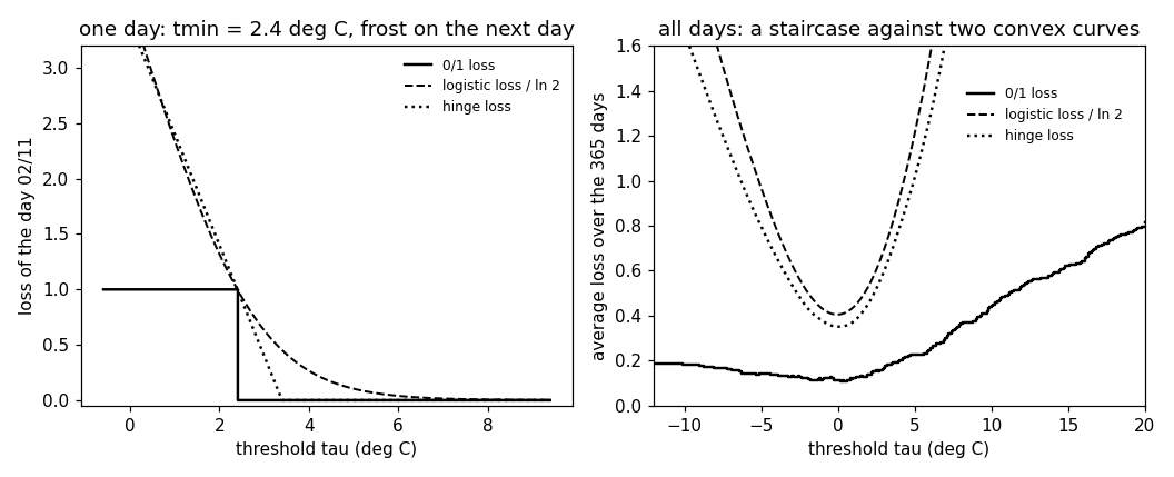
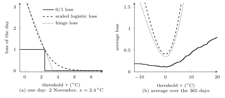
B-stairFig. 1 shows both obstacles in the frost warning of the opening. Each of the $m = 365$ days of $2024$ at Krems is a data point whose single feature $x$ is the lowest temperature of the day and whose label is $y = +1$ if the lowest temperature of the following day is below $0\,^{\circ}\mathrm{C}$ (frost) and $y = -1$ otherwise. Frost follows $68$ of the $365$ days. The warning compares the day's lowest temperature with a threshold $\tau$: the hypothesis $h(x) = \tau - x$ predicts frost when it is positive, and the single model parameter $\tau$ selects a classifier from the hypothesis space of all thresholds. The $0/1$ loss of one day is a step in $\tau$, from $1$ to $0$ at the day's temperature, and the average over the year is a staircase with $195$ steps, one at each distinct temperature. Its smallest value, $40/365 = 0.110$, is attained by every threshold strictly between $0.2$ and $0.3$ and between $0.4$ and $0.6\,^{\circ}\mathrm{C}$: the set of minimizers is not a single point, and the slope of the staircase is zero at every threshold that is not a jump. A warning that never predicts frost has average $0/1$ loss $68/365 = 0.186$, and one that always predicts frost has $0.814$.
B-smoothPractical classification methods replace the $0/1$ loss in ERM by a surrogate loss function that is convex in $h({\mathbf x})$ and an upper bound on the $0/1$ loss (Shalev-Shwartz and Ben-David, 2014, Sect. 12.3). The hinge loss $\max\{0, 1 - y \cdot h({\mathbf x})\}$, which gives the support vector machine (SVM), lies on or above the $0/1$ loss for every margin (Shalev-Shwartz and Ben-David, 2014, Sect. 12.3). The logistic loss $\ln(1 + \exp(-y \cdot h({\mathbf x})))$, which gives logistic regression, equals $\ln 2 \approx 0.69$ at margin $0$ and is an upper bound only after division by $\ln 2$. Scaling a surrogate so that it passes through $1$ at margin $0$ is the usual convention when loss functions are compared (Bishop, 2006, Fig. 7.5; Hastie et al., 2009, Sect. 10.6). Because the surrogate is an upper bound, the risk of any hypothesis under the $0/1$ loss is at most its risk under the surrogate, so a hypothesis with a small surrogate risk misclassifies rarely (Shalev-Shwartz and Ben-David, 2014, Sect. 12.3). Both surrogates are also calibrated for classification: for a convex function of the margin that is differentiable at $0$ with a negative derivative there, every sequence of hypotheses whose surrogate risk tends to its smallest possible value has a $0/1$ risk that tends to the Bayes risk (Bartlett et al., 2006, Thms. 1 and 6). Over all functions of ${\mathbf x}$, the hinge loss is minimized by the sign of $\mathbb{P}\left(y = +1 \mid {\mathbf x}\right) - 1/2$ and the logistic loss by the logarithm of the odds of $y = +1$, and the sign of either minimizer is the classifier with the Bayes risk (Hastie et al., 2009, Table 12.1). Unlike the $0/1$ loss, a surrogate changes when $h$ is multiplied by a positive number, so it depends on the scale of $h$ and not only on its sign.
For the frost warning, the average logistic loss divided by
$\ln 2$ and the average hinge loss are convex
functions of the threshold that lie above the staircase
everywhere (Fig. 1). Each has a
single minimizer, $\tau = -0.04\,^{\circ}\mathrm{C}$ for
the logistic loss and $0.06\,^{\circ}\mathrm{C}$ for the
hinge loss, and at both the average $0/1$ loss is
$41/365 = 0.112$, one day more than the smallest value of the
staircase. At the minimizer of the logistic loss, the average
logistic loss divided by $\ln 2$ is $0.405$ for $h$,
$0.333$ for $h/2$, and $0.670$ for $2h$, while
the average $0/1$ loss is the same for all three.
pythondemos/zerooneloss.py
Synonyms: misclassification loss, zero-one loss.
See also: loss, loss function, classification, binary classification, classifier, accuracy, training error, risk, Bayes risk, margin, hinge loss, logistic loss, empirical risk minimization, support vector machine, logistic regression, confusion matrix, imbalanced data.
@misc{dictml_zerooneloss,
  author = {Jung, Alexander},
  editor = {Olioumtsevits, Konstantina and Schnoor, Ekkehard},
  title = {$\bf 0/1$ loss},
  howpublished = {Dictionary of Applied Machine Learning (course edition)},
  year = {2026},
  doi = {10.5281/zenodo.21569296},
  note = {ISBN 978-952-64-3013-3, CC BY 4.0, retrieved 2026-11-20},
  url = {https://dictionaryofml.org/terms/zerooneloss.html}
}