B-plot writes when the script runsDictionary of Applied Machine Learning · $\bf 0/1$ loss
Updated on 2026-11-19
Numerical companion to the entry $\bf 0/1$ loss: it recomputes what the entry states and prints one line per check
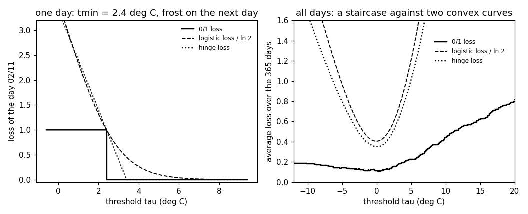
Numerical companion to the glossary entry 'zerooneloss'. Each of the 365 days of 2024 at Krems (GeoSphere station 3805) is a data point: its feature x is the lowest temperature of the day, its label y is +1 if the lowest temperature of the following day is below zero (frost) and -1 otherwise. A frost warning compares today's lowest temperature with a threshold tau: the real-valued hypothesis h(x) = tau - x predicts frost when it is positive, and the thresholds form a one-parameter family of classifiers.
Run it without installing anything:uv run https://dictionaryofml.org/terms/zerooneloss.py
uv downloads this script and the pinned NumPy and Matplotlib it needs, then runs it; the script fetches any input file it uses. To keep the output files, download zerooneloss.py into a folder and run uv run zerooneloss.py there. With NumPy and Matplotlib already installed, python3 zerooneloss.py, from any directory — it writes its output files into the current directory. Fixed seeds, so the printed numbers reproduce exactly. Download zerooneloss.py · Notebook · Open in Colab
Before running a downloaded copy, scan it: uvx bandit -q -t B102,B307,B602,B605 zerooneloss.py (B102,B307,B602,B605 are the exec, eval and shell checks of bandit) reports nothing: the script runs no shell command and evaluates no generated code.
One cell per block of the script: the code, and what that code printed when it last ran here
"""The 0/1 loss of a frost warning at Krems an der Donau: a staircase in
the threshold against the smooth curve of the logistic loss.

Purpose
-------
Numerical companion to the glossary entry 'zerooneloss'.  Each of the
365 days of 2024 at Krems (GeoSphere station 3805) is a data point: its
feature x is the lowest temperature of the day, its label y is +1 if the
lowest temperature of the following day is below zero (frost) and -1
otherwise.  A frost warning compares today's lowest temperature with a
threshold tau: the real-valued hypothesis h(x) = tau - x predicts frost
when it is positive, and the thresholds form a one-parameter family of
classifiers.

The demo checks the entry's claims: the 0/1 loss of one day is a step
in tau, while its logistic loss (divided by ln 2) and its hinge loss
are convex curves that lie on or above the step and equal 1 where the
step jumps; the average 0/1 loss over the year is piecewise constant in
tau, equal to one minus the accuracy, with a flat set of minimizers and
a zero slope wherever the slope exists; the average logistic loss and
the average hinge loss are convex in tau, lie above the staircase and
have one minimizer each, at which the staircase is close to its
minimum; and the 0/1 loss does not change when the hypothesis is
multiplied by a positive factor, while the logistic loss does.

Deterministic: no random numbers.  Self-contained: numpy + matplotlib
only; the GeoSphere download falls back to the committed CSV.

Blocks
------
[B-data]    Download the daily lowest temperature of 2024 at Krems or
            read the committed copy; 366 days give 365 (feature, label)
            pairs, and the frost days are counted.
[B-oneday]  The three losses of one day, the first day of autumn that was
            followed by frost, as functions of the threshold tau: the 0/1
            loss jumps once, at tau equal to the day's temperature; the
            logistic loss / ln 2 and the hinge loss decrease, equal 1 at
            the jump and never fall below the 0/1 loss.
[B-stair]   The average 0/1 loss over the 365 days is a staircase in tau:
            constant between consecutive distinct temperatures, one minus
            the accuracy, with the never-frost and always-frost baselines
            at its two ends, a flat interval of minimizers, and a
            difference quotient of exactly zero away from the jumps.
[B-smooth]  The average logistic loss / ln 2 and the average hinge loss
            are convex in tau and lie above the staircase; each has one
            minimizer, and the average 0/1 loss there is compared with
            the smallest average 0/1 loss.
[B-scale]   Multiplying the hypothesis by a positive factor leaves the
            average 0/1 loss unchanged and changes the average logistic
            loss.
[B-plot]    CSVs for the figure and the matplotlib preview.

Outputs
-------
zerooneloss_weather.csv : date, tmin (committed copy of the download).
zerooneloss_oneday.csv  : tau, zo, log2, hinge for the one day.
zerooneloss_stair.csv   : tau, zo: the staircase of the average 0/1 loss
                          (one row per step, for a const plot).
zerooneloss_curves.csv  : tau, log2, hinge: the two average surrogate
                          losses on a grid.
zerooneloss.png         : matplotlib preview (checking only).
"""

# /// script
# requires-python = ">=3.10"
# dependencies = ["matplotlib==3.10.7", "numpy==2.3.4"]
# ///

import json
import urllib.request
from pathlib import Path

import numpy as np
import matplotlib

matplotlib.use("Agg")
import matplotlib.pyplot as plt

OUT_DIR = Path(__file__).parent
LN2 = float(np.log(2.0))

report = []


def check(name, ok):
    report.append((name, bool(ok)))
    print(f"  [{'ok' if ok else 'FAIL'}] {name}")
Download the daily lowest temperature of 2024 at Krems or read the committed copy; 366 days give 365 (feature, label) pairs, and the frost days are counted.
print("[B-data] daily lowest temperature at Krems, 2024")
URL = ("https://dataset.api.hub.geosphere.at/v1/station/historical/"
       "klima-v2-1d?parameters=tlmin&station_ids=3805"
       "&start=2024-01-01&end=2024-12-31")
CSV = OUT_DIR / "zerooneloss_weather.csv"
try:
    with urllib.request.urlopen(URL, timeout=120) as resp:
        payload = json.load(resp)
    params = payload["features"][0]["properties"]["parameters"]
    records = [(stamp[:10], lo) for stamp, lo in
               zip(payload["timestamps"], params["tlmin"]["data"])]
    if any(lo is None for _, lo in records):
        raise OSError("a day is missing its temperature")
    with open(CSV, "w") as fh:
        fh.write("date,tmin\n")
        for day, lo in records:
            fh.write(f"{day},{lo}\n")
    print(f"    downloaded {len(records)} days")
except OSError as err:
    print(f"    download failed ({err}); reading the committed CSV")
    rows = CSV.read_text().strip().splitlines()[1:]
    records = [(d, float(a)) for d, a in (r.split(",") for r in rows)]

check("[B-data] 366 days for 2024", len(records) == 366)
dates = [d for d, _ in records]
tlmin = np.array([lo for _, lo in records], dtype=float)
x = tlmin[:-1]                                  # today's lowest temperature
y = np.where(tlmin[1:] < 0.0, 1.0, -1.0)        # +1: frost on the next day
m = len(x)
n_frost = int(np.sum(y > 0))
check(f"[B-data] m = {m} data points; frost follows {n_frost} of them "
      f"(fraction {n_frost / m:.3f})", m == 365 and 0 < n_frost < m)


# ---- the three losses of one data point along the threshold family
def zo_loss(margin):
    """0/1 loss: 1 unless the margin is positive."""
    return np.where(margin > 0.0, 0.0, 1.0)


def log2_loss(margin):
    """Logistic loss divided by ln 2, so that it equals 1 at margin 0."""
    return np.logaddexp(0.0, -margin) / LN2


def hinge_loss(margin):
    return np.maximum(0.0, 1.0 - margin)


def margins(tau, scale=1.0):
    """Margins y * h(x) of all days for the hypothesis h(x) = scale*(tau-x)."""
    return y * scale * (tau - x)


def avg_zo(tau, scale=1.0):
    return float(np.mean(zo_loss(margins(tau, scale))))


def avg_log2(tau, scale=1.0):
    return float(np.mean(log2_loss(margins(tau, scale))))


def avg_hinge(tau, scale=1.0):
    return float(np.mean(hinge_loss(margins(tau, scale))))
[B-data] daily lowest temperature at Krems, 2024
    downloaded 366 days
  [ok] [B-data] 366 days for 2024
  [ok] [B-data] m = 365 data points; frost follows 68 of them (fraction 0.186)
The three losses of one day, the first day of autumn that was followed by frost, as functions of the threshold tau: the 0/1 loss jumps once, at tau equal to the day's temperature; the logistic loss / ln 2 and the hinge loss decrease, equal 1 at the jump and never fall below the 0/1 loss.
print("[B-oneday] the losses of one day as functions of the threshold")
autumn = [i for i in range(m) if dates[i] >= "2024-09-01" and y[i] > 0]
i_day = autumn[0]
x_day, y_day = float(x[i_day]), float(y[i_day])
day_label = dates[i_day][8:10] + "/" + dates[i_day][5:7]
check(f"[B-oneday] the first autumn day followed by frost is {day_label}, "
      f"with lowest temperature {x_day:.1f} deg C", y_day > 0)
tau_day = np.linspace(x_day - 3.0, x_day + 7.0, 1001)
mg_day = y_day * (tau_day - x_day)
zo_day, lg_day, hg_day = zo_loss(mg_day), log2_loss(mg_day), hinge_loss(mg_day)
check("[B-oneday] its 0/1 loss is 1 for every threshold at or below the "
      "day's temperature and 0 above it",
      np.all(zo_day[tau_day <= x_day] == 1.0)
      and np.all(zo_day[tau_day > x_day] == 0.0))
check("[B-oneday] the logistic loss / ln 2 and the hinge loss both equal 1 "
      "at the jump (margin 0)",
      abs(log2_loss(0.0) - 1.0) < 1e-12 and hinge_loss(0.0) == 1.0)
check("[B-oneday] both surrogates lie on or above the 0/1 loss at every "
      "threshold and decrease with it",
      np.all(lg_day >= zo_day - 1e-12) and np.all(hg_day >= zo_day - 1e-12)
      and np.all(np.diff(lg_day) < 0) and np.all(np.diff(hg_day) <= 0))
check(f"[B-oneday] one degree above the jump the 0/1 loss is 0 while the "
      f"logistic loss / ln 2 is {log2_loss(1.0):.3f} and the hinge loss 0",
      zo_loss(1.0) == 0.0 and 0.4 < log2_loss(1.0) < 0.5 and hinge_loss(1.0) == 0)
[B-oneday] the losses of one day as functions of the threshold
  [ok] [B-oneday] the first autumn day followed by frost is 02/11, with lowest temperature 2.4 deg C
  [ok] [B-oneday] its 0/1 loss is 1 for every threshold at or below the day's temperature and 0 above it
  [ok] [B-oneday] the logistic loss / ln 2 and the hinge loss both equal 1 at the jump (margin 0)
  [ok] [B-oneday] both surrogates lie on or above the 0/1 loss at every threshold and decrease with it
  [ok] [B-oneday] one degree above the jump the 0/1 loss is 0 while the logistic loss / ln 2 is 0.452 and the hinge loss 0
The average 0/1 loss over the 365 days is a staircase in tau: constant between consecutive distinct temperatures, one minus the accuracy, with the never-frost and always-frost baselines at its two ends, a flat interval of minimizers, and a difference quotient of exactly zero away from the jumps.
print("[B-stair] the average 0/1 loss over the year is a staircase")
xs = np.unique(x)                               # the jump positions
n_steps = len(xs)
# value of the staircase on the open interval (xs[k], xs[k+1]); the last
# entry is the value above the largest temperature
mids = np.concatenate([(xs[:-1] + xs[1:]) / 2.0, [xs[-1] + 1.0]])
stair = np.array([avg_zo(t) for t in mids])
below = avg_zo(xs[0] - 1.0)                     # never predict frost
check(f"[B-stair] the staircase has {n_steps} jumps, one per distinct "
      f"temperature among the {m} days", n_steps < m)
probe = np.concatenate([(xs[:-1] + 0.25 * (xs[1:] - xs[:-1])),
                        (xs[:-1] + 0.75 * (xs[1:] - xs[:-1]))])
check("[B-stair] between two consecutive temperatures the average 0/1 loss "
      "is constant",
      all(avg_zo(t) == stair[k] for k, t in enumerate(probe[: n_steps - 1]))
      and all(avg_zo(t) == stair[k]
              for k, t in enumerate(probe[n_steps - 1:])))
acc_at = [np.mean(np.where(tau - x > 0, 1.0, -1.0) == y) for tau in mids]
check("[B-stair] it equals one minus the accuracy at every threshold",
      np.allclose(stair, 1.0 - np.array(acc_at)))
check(f"[B-stair] below every temperature the warning never predicts frost "
      f"and the average 0/1 loss is the frost fraction {below:.3f}; above "
      f"every temperature it always predicts frost and the loss is "
      f"{stair[-1]:.3f}",
      abs(below - n_frost / m) < 1e-12 and abs(stair[-1] - (1 - n_frost / m)) < 1e-12)
zo_min = float(stair.min())
flat = np.flatnonzero(stair == zo_min)
# the minimizers form open intervals between consecutive temperatures;
# adjacent steps are collected into runs, each named by its two ends
runs, start = [], flat[0]
for a, b in zip(flat, flat[1:]):
    if b != a + 1:
        runs.append((float(xs[start]), float(xs[a + 1])))
        start = b
runs.append((float(xs[start]), float(xs[flat[-1] + 1])))
lo_tau, hi_tau = runs[0][0], runs[-1][1]
spans = " and ".join(f"({a:.1f}, {b:.1f})" for a, b in runs)
check(f"[B-stair] the smallest average 0/1 loss is {zo_min:.3f} "
      f"({int(round(zo_min * m))} of {m} days wrong, accuracy "
      f"{1 - zo_min:.3f}), reached by every threshold in the open "
      f"interval(s) {spans} deg C: {len(runs)} interval(s)",
      zo_min < below and all(b > a for a, b in runs))
check(f"[B-stair] a threshold of exactly {lo_tau:.1f} deg C does worse "
      f"({avg_zo(lo_tau):.3f}): a day at margin 0 counts as misclassified",
      avg_zo(lo_tau) > zo_min)
grid = np.linspace(-12.0, 20.0, 641)
away = grid[np.min(np.abs(grid[:, None] - xs[None, :]), axis=1) > 1e-3]
delta = 5e-4
check("[B-stair] the difference quotient of the average 0/1 loss is exactly "
      "zero at every grid point away from the jumps",
      all(avg_zo(t + delta) - avg_zo(t) == 0.0 for t in away))
check(f"[B-stair] the staircase takes {len(np.unique(stair))} distinct "
      f"values, each a multiple of 1/{m}",
      np.allclose(stair * m, np.round(stair * m)))
[B-stair] the average 0/1 loss over the year is a staircase
  [ok] [B-stair] the staircase has 195 jumps, one per distinct temperature among the 365 days
  [ok] [B-stair] between two consecutive temperatures the average 0/1 loss is constant
  [ok] [B-stair] it equals one minus the accuracy at every threshold
  [ok] [B-stair] below every temperature the warning never predicts frost and the average 0/1 loss is the frost fraction 0.186; above every temperature it always predicts frost and the loss is 0.814
  [ok] [B-stair] the smallest average 0/1 loss is 0.110 (40 of 365 days wrong, accuracy 0.890), reached by every threshold in the open interval(s) (0.2, 0.3) and (0.4, 0.6) deg C: 2 interval(s)
  [ok] [B-stair] a threshold of exactly 0.2 deg C does worse (0.115): a day at margin 0 counts as misclassified
  [ok] [B-stair] the difference quotient of the average 0/1 loss is exactly zero at every grid point away from the jumps
  [ok] [B-stair] the staircase takes 146 distinct values, each a multiple of 1/365
The average logistic loss / ln 2 and the average hinge loss are convex in tau and lie above the staircase; each has one minimizer, and the average 0/1 loss there is compared with the smallest average 0/1 loss.
def argmin_convex(f, lo, hi, iters=200):
    """Ternary search for the minimizer of a convex function on [lo, hi]."""
    for _ in range(iters):
        a, b = lo + (hi - lo) / 3.0, hi - (hi - lo) / 3.0
        if f(a) < f(b):
            hi = b
        else:
            lo = a
    return (lo + hi) / 2.0


print("[B-smooth] the average logistic and hinge losses are convex curves")
lg_grid = np.array([avg_log2(t) for t in grid])
hg_grid = np.array([avg_hinge(t) for t in grid])
zo_grid = np.array([avg_zo(t) for t in grid])
check("[B-smooth] both averages are convex in the threshold (second "
      "differences nonnegative on the grid)",
      np.all(np.diff(lg_grid, 2) >= -1e-10)
      and np.all(np.diff(hg_grid, 2) >= -1e-10))
check("[B-smooth] both averages lie on or above the average 0/1 loss at "
      "every grid point",
      np.all(lg_grid >= zo_grid - 1e-12) and np.all(hg_grid >= zo_grid - 1e-12))
tau_log = argmin_convex(avg_log2, -12.0, 20.0)
tau_hinge = argmin_convex(avg_hinge, -12.0, 20.0)
check(f"[B-smooth] the average logistic loss / ln 2 has its minimum "
      f"{avg_log2(tau_log):.3f} at tau = {tau_log:.2f} deg C, where the "
      f"average 0/1 loss is {avg_zo(tau_log):.3f}",
      lo_tau - 3.0 < tau_log < hi_tau + 3.0)
check(f"[B-smooth] the average hinge loss has its minimum "
      f"{avg_hinge(tau_hinge):.3f} at tau = {tau_hinge:.2f} deg C, where "
      f"the average 0/1 loss is {avg_zo(tau_hinge):.3f}",
      lo_tau - 3.0 < tau_hinge < hi_tau + 3.0)
check(f"[B-smooth] the staircase at the two surrogate minimizers "
      f"({avg_zo(tau_log):.3f}, {avg_zo(tau_hinge):.3f}) is within "
      f"{3 / m:.3f} (three days) of its minimum {zo_min:.3f}",
      avg_zo(tau_log) <= zo_min + 3 / m + 1e-12
      and avg_zo(tau_hinge) <= zo_min + 3 / m + 1e-12)
check("[B-smooth] the slope of the average logistic loss is negative one "
      "degree below its minimizer and positive one degree above it",
      avg_log2(tau_log - 1.0 + 1e-3) < avg_log2(tau_log - 1.0)
      and avg_log2(tau_log + 1.0 + 1e-3) > avg_log2(tau_log + 1.0))
[B-smooth] the average logistic and hinge losses are convex curves
  [ok] [B-smooth] both averages are convex in the threshold (second differences nonnegative on the grid)
  [ok] [B-smooth] both averages lie on or above the average 0/1 loss at every grid point
  [ok] [B-smooth] the average logistic loss / ln 2 has its minimum 0.405 at tau = -0.04 deg C, where the average 0/1 loss is 0.112
  [ok] [B-smooth] the average hinge loss has its minimum 0.352 at tau = 0.06 deg C, where the average 0/1 loss is 0.112
  [ok] [B-smooth] the staircase at the two surrogate minimizers (0.112, 0.112) is within 0.008 (three days) of its minimum 0.110
  [ok] [B-smooth] the slope of the average logistic loss is negative one degree below its minimizer and positive one degree above it
Multiplying the hypothesis by a positive factor leaves the average 0/1 loss unchanged and changes the average logistic loss.
print("[B-scale] the hypothesis multiplied by a positive factor")
check("[B-scale] the average 0/1 loss is the same for h, h/2 and 2h at "
      "every grid point",
      all(avg_zo(t, 0.5) == avg_zo(t) == avg_zo(t, 2.0) for t in grid))
check(f"[B-scale] the average logistic loss / ln 2 at tau = {tau_log:.2f} "
      f"changes: {avg_log2(tau_log, 0.5):.3f} for h/2, "
      f"{avg_log2(tau_log):.3f} for h, {avg_log2(tau_log, 2.0):.3f} for 2h",
      avg_log2(tau_log, 0.5) != avg_log2(tau_log)
      != avg_log2(tau_log, 2.0))
[B-scale] the hypothesis multiplied by a positive factor
  [ok] [B-scale] the average 0/1 loss is the same for h, h/2 and 2h at every grid point
  [ok] [B-scale] the average logistic loss / ln 2 at tau = -0.04 changes: 0.333 for h/2, 0.405 for h, 0.670 for 2h
CSVs for the figure and the matplotlib preview.
print("[B-plot] CSVs and preview")
with open(OUT_DIR / "zerooneloss_oneday.csv", "w") as fh:
    fh.write("tau,zo,log2,hinge\n")
    for t, a, b, c in zip(tau_day, zo_day, lg_day, hg_day):
        fh.write(f"{t:.4f},{a:.0f},{b:.6f},{c:.6f}\n")
with open(OUT_DIR / "zerooneloss_stair.csv", "w") as fh:
    fh.write("tau,zo\n")
    fh.write(f"{grid[0]:.4f},{below:.6f}\n")
    for t, v in zip(xs, stair):
        fh.write(f"{t:.4f},{v:.6f}\n")
    fh.write(f"{grid[-1]:.4f},{stair[-1]:.6f}\n")
with open(OUT_DIR / "zerooneloss_curves.csv", "w") as fh:
    fh.write("tau,log2,hinge\n")
    for t, a, b in zip(grid, lg_grid, hg_grid):
        fh.write(f"{t:.4f},{a:.6f},{b:.6f}\n")
check(f"[B-plot] the staircase CSV has {n_steps + 2} rows, the curves CSV "
      f"{len(grid)}", True)

fig, (ax1, ax2) = plt.subplots(1, 2, figsize=(9.6, 3.9))
ax1.step(tau_day, zo_day, where="post", color="black", lw=1.6,
         label="0/1 loss")
ax1.plot(tau_day, lg_day, "k--", lw=1.3, label="logistic loss / ln 2")
ax1.plot(tau_day, hg_day, "k:", lw=1.6, label="hinge loss")
ax1.set_xlabel("threshold tau (deg C)")
ax1.set_ylabel(f"loss of the day {day_label}")
ax1.set_title(f"one day: tmin = {x_day:.1f} deg C, frost on the next day")
ax1.set_ylim(-0.05, 3.2)
ax1.legend(frameon=False, fontsize=8)
stair_x = np.concatenate([[grid[0]], xs, [grid[-1]]])
stair_y = np.concatenate([[below], stair, [stair[-1]]])
ax2.step(stair_x, stair_y, where="post", color="black", lw=1.6,
         label="0/1 loss")
ax2.plot(grid, lg_grid, "k--", lw=1.3, label="logistic loss / ln 2")
ax2.plot(grid, hg_grid, "k:", lw=1.6, label="hinge loss")
ax2.set_xlabel("threshold tau (deg C)")
ax2.set_ylabel(f"average loss over the {m} days")
ax2.set_title("all days: a staircase against two convex curves")
ax2.set_xlim(grid[0], grid[-1])
ax2.set_ylim(0.0, 1.6)
ax2.legend(frameon=False, fontsize=8, loc="upper right",
           bbox_to_anchor=(0.98, 0.92))
fig.tight_layout()
fig.savefig(OUT_DIR / "zerooneloss.png", dpi=110)

n_ok = sum(ok for _, ok in report)
print(f"\n{n_ok}/{len(report)} checks pass")
if n_ok != len(report):
    raise SystemExit(1)
[B-plot] CSVs and preview
  [ok] [B-plot] the staircase CSV has 197 rows, the curves CSV 641

24/24 checks pass
B-plot writes when the script runs