decisionboundary.py, which recomputes what the entry states: the script block by block · open in ColabDictionary of Applied Machine Learning: 114 machine-learning terms, each with a definition, a figure, citations and a Python demo · All terms · Demos · Start here
Updated on 2026-10-31
Readiness 85/100
See also hypothesis feature vector
decisionboundary.py, which recomputes what the entry states: the script block by block · open in ColabConsider a hypothesis $h\colon\mathcal{X}\rightarrow\mathcal{Y}$ whose finite label space $\mathcal{Y}$ represents different classes. Its decision boundary consists of those feature vectors that are arbitrarily close to two or more different decision regions. More precisely, ${\mathbf x}\in\mathcal{X}$ lies on the decision boundary if every neighborhood of ${\mathbf x}$ contains feature vectors ${\mathbf x}'$ and ${\mathbf x}''$ such that $h({\mathbf x}')\neqh({\mathbf x}'')$. Thus, arbitrarily small perturbations near the decision boundary can result in different predicted labels (or classes).
A common construction of a classifier is by thresholding a real-valued scoring function $g\colon\mathcal{X}\rightarrow\mathbb{R}$. The classifier assigns different labels according to whether $g({\mathbf x})$ lies below or above a threshold $c$. If $g$ is continuous, its decision boundary is the level set $\{{\mathbf x}:g({\mathbf x})=c\}$, provided that $g$ takes values on both sides of $c$ arbitrarily close to every point in this set. For a linear classifier with $g({\mathbf x})={\mathbf w}^{\top}{\mathbf x}$ and ${\mathbf w}\neq\mathbf{0}$, this level set is the hyperplane ${\mathbf w}^{\top}{\mathbf x}=c$, whose normal vector is ${\mathbf w}$ (Bishop, 2006, Sect. 4.1; Hastie et al., 2009, Ch. 4).
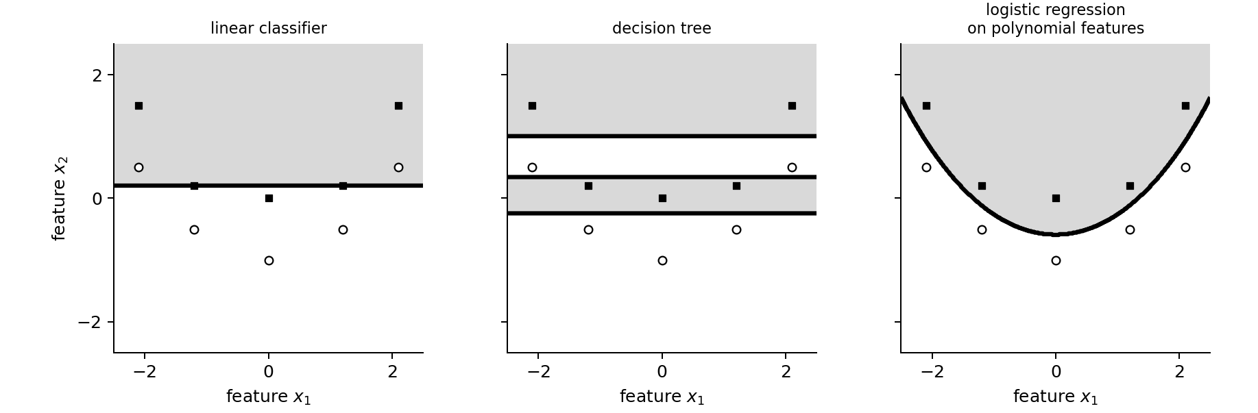
Fig. 1 shows that the geometry of a
decision boundary depends on the model. A
linear classifier produces a straight boundary, a decision tree
produces an axis-aligned, piecewise constant boundary, and
logistic regression applied to polynomial features can produce a
curved boundary.
pythondemos/decisionboundary.py
See also: hypothesis, feature vector, label space, boundary, decision region, neighborhood.
@misc{dictml_decisionboundary,
  author = {Jung, Alexander},
  editor = {Olioumtsevits, Konstantina and Schnoor, Ekkehard},
  title = {decision boundary},
  howpublished = {Dictionary of Applied Machine Learning (course edition)},
  year = {2026},
  doi = {10.5281/zenodo.21569296},
  note = {ISBN 978-952-64-3013-3, CC BY 4.0, retrieved 2026-11-02},
  url = {https://dictionaryofml.org/terms/decisionboundary.html}
}