mse.py, which recomputes what the entry states: the script block by block · open in ColabDictionary of Applied Machine Learning: 147 machine-learning terms, each with a definition, a figure, citations and a Python demo · All terms · Demos · Start here
Updated on 2026-11-20
Readiness 88/100
The mean squared error (MSE) of a hypothesis is the average of its squared error loss, the squared difference between the label of a data point and the prediction for it. The average is either an expectation under a probabilistic model for the data, the independent and identically distributed assumption (i.i.d. assumption), which makes the MSE the risk under the squared error loss, or the average over the data points of a dataset, which makes it the empirical risk, the training error or the validation error. The two readings coincide for the empirical distribution of the dataset, which assigns the same probability to each of its data points. When the i.i.d. assumption holds, the average over a dataset estimates the expectation and improves with the sample size. The root MSE, its square root, is measured in the unit of the label.
mse.py, which recomputes what the entry states: the script block by block · open in ColabB-dataConsider a hypothesis $h$ that predicts the maximum daytime temperature of a day at Krems an der Donau (Austria) from its morning minimum. A weather service that uses it reports one number for how far the predictions are off on average, and the MSE is that number: the average of the squared error loss, the squared difference between the label of a data point and the prediction for it. The word average has two readings here, and the MSE is defined in both.
B-averageThe first reading needs a probabilistic model for how the data come about. The independent and identically distributed assumption (i.i.d. assumption) is the simplest one: it treats the daily weather measurements as realizations of independent and identically distributed (i.i.d.) random variables (RVs), so that each day, a data point with feature vector ${\mathbf x}$ and label $y$, is an independent draw from one probability distribution $\mathbb{P}$ that does not change from day to day. Under this model, the MSE of $h$ is the expectation of its squared error loss, \begin{equation} \label{equ_mse_expectation_dict} \bar{L} \big( h \big) := \mathbb{E} \big\{ \big(y - h({\mathbf x})\big)^{2} \big\} \text{,} \end{equation} which is the risk of $h$ under the squared error loss (Hastie et al., 2009, Sect. 2.4). The expectation \(\eqref{equ_mse_expectation_dict}\) is taken over the probability distribution $\mathbb{P}$ of the data point, which the i.i.d. assumption postulates but does not specify: in a machine learning (ML) application, $\mathbb{P}$ is unknown. What can be computed is the MSE on a dataset $\mathcal{D} = \{({\mathbf x}^{(1)}, y^{(1)}), \ldots, ({\mathbf x}^{(m)}, y^{(m)})\}$ of sample size $m$, the average of the squared error loss over its data points, \begin{equation} \label{equ_mse_average_dict} \widehat{L}\big(h|\mathcal{D}\big) := \frac{1}{m} \sum_{r=1}^{m} \big(y^{(r)} - h({\mathbf x}^{(r)})\big)^{2} \text{,} \end{equation} which is the empirical risk of $h$ on $\mathcal{D}$ under the squared error loss. It is the training error when $\mathcal{D}$ is the training set and the validation error when $\mathcal{D}$ is the validation set. For a linear model learned by least squares on the $365$ days of $2023$ at Krems, the MSE \(\eqref{equ_mse_average_dict}\) is $21.1$ on those days and $19.2$ on the $366$ days of $2024$, in squared degrees. Its square root, the root MSE of $4.4$ degrees, has the unit of the label.
B-robustThe two definitions are one definition applied to two
probability distributions. The empirical distribution
$\mathbb{P}^{(\mathcal{D})}$ of the dataset $\mathcal{D}$ assigns the
probability $1/m$ to each of its data points.
The expectation of the squared error loss under
$\mathbb{P}^{(\mathcal{D})}$ is therefore a sum of $m$ terms
with weight $1/m$ each,
\begin{equation}
\label{equ_mse_empdist_dict}
\mathbb{E}_{({\mathbf x}, y) \sim \mathbb{P}^{(\mathcal{D})}}
\big\{ \big(y - h({\mathbf x})\big)^{2} \big\}
= \widehat{L}\big(h|\mathcal{D}\big) \text{.}
\end{equation}
By the identity \(\eqref{equ_mse_empdist_dict}\), the average
\(\eqref{equ_mse_average_dict}\) is the expectation
\(\eqref{equ_mse_expectation_dict}\) with the
empirical distribution of $\mathcal{D}$ in place of $\mathbb{P}$.
Every statement about the MSE as an expectation then holds for
the average with $\mathbb{P}^{(\mathcal{D})}$ in that role, such as its
split into the variance of the label around its
conditional mean and the squared deviation of $h$
from that mean (Bishop, 2006, Sect. 1.5.5).
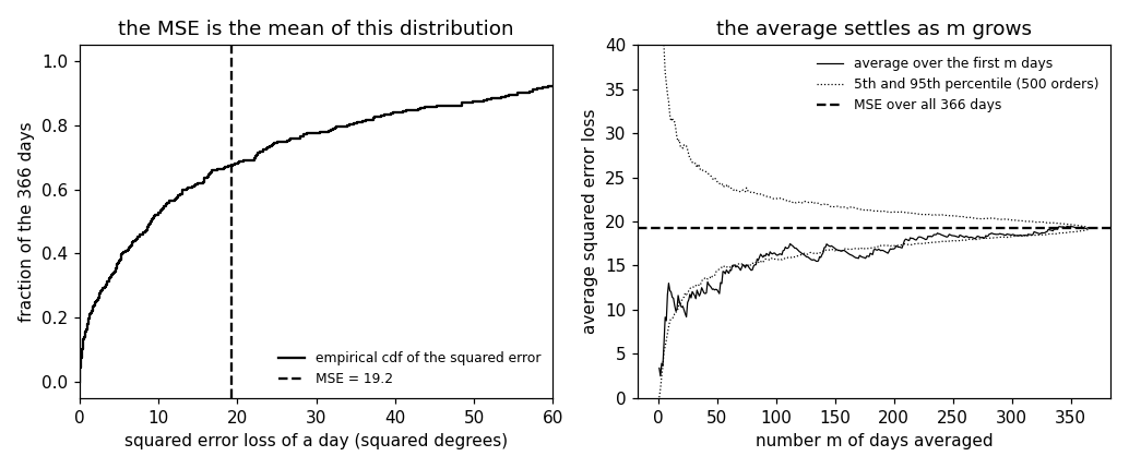
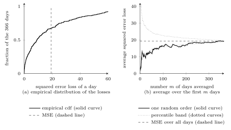
Fig. 1(a) draws the empirical distribution of
the squared errors of the $366$ days of $2024$. Its mean is
the MSE $19.2$, while its median is $9.1$ and two thirds of
the days have a loss below the MSE: a few far-off days weigh
heavily in a squared average. Conversely, when the
data points of $\mathcal{D}$ are realizations of i.i.d.
RVs with probability distribution $\mathbb{P}$, the average
\(\eqref{equ_mse_average_dict}\) is an estimate of the expectation
\(\eqref{equ_mse_expectation_dict}\) that improves with the
sample size $m$ by the law of large numbers. Fig. 1(b)
shows this for the days of $2024$ in a random order: over the first
$30$ days, the average lies between $12.6$ and $26.7$ in nine of
ten orders, over the first $180$ days between $17.0$ and $21.3$.
How far the training error can lie from the risk is the
subject of generalization.
pythondemos/mse.py
@misc{dictml_mse,
  author = {Jung, Alexander},
  editor = {Olioumtsevits, Konstantina and Schnoor, Ekkehard},
  title = {mean squared error (MSE)},
  howpublished = {Dictionary of Applied Machine Learning (course edition)},
  year = {2026},
  doi = {10.5281/zenodo.21569296},
  note = {ISBN 978-952-64-3013-3, CC BY 4.0, retrieved 2026-11-20},
  url = {https://dictionaryofml.org/terms/mse.html}
}