pythondemos/samplesize.pyDictionary of Applied Machine Learning
Updated on 2026-10-14
See also data point dataset independent and identically distributed assumption validation error overfitting
The sample size is the number $\samplesize$ of data points in a sample. Many machine learning (ML) methods model the data points as realizations of independent and identically distributed (i.i.d.) random variables (RVs) and judge a hypothesis by its expected loss, the risk; since the probability distribution is unknown, the risk is estimated by the average loss on the sample, for training by empirical risk minimization (ERM) and for validation. How close that average is to the risk depends on the sample size. A concentration inequality such as Hoeffding's inequality bounds the deviation of the average from the risk and turns a required accuracy $\epsilon$ and confidence $1 - \delta$ into a sample size of order $\log(1/\delta) / \epsilon^{2}$ for validation; for training, the sample size must also be compared with the size of the model. For data points recorded in sequence, autocorrelation lowers the effective sample size. The same reasoning sizes the sample for a statistical test, such as whether two features are correlated: the sample size needed to detect a correlation grows as the inverse square of that correlation.
B-riskA frost warning for Krems an der Donau predicts, from the minimum and the maximum temperature of a day, whether the next day brings frost. Whether a hypothesis $\hypothesis$ for this task is any good is judged by its expected loss, the risk $\risk{\hypothesis} = \expect \{ \lossfunc{\datapoint}{\hypothesis} \}$, where the expectation is over a data point $\datapoint$ drawn from the probability distribution $\probdist^{(\datapoint)}$ of the days. Many machine learning (ML) methods use the independent and identically distributed assumption (i.i.d. assumption): the data points are realizations of independent and identically distributed (i.i.d.) random variables (RVs) $\datapoint^{(1)}, \ldots, \datapoint^{(\samplesize)} \sim \probdist^{(\datapoint)}$. In practice, $\probdist^{(\datapoint)}$ is unknown, and a method observes only these $\samplesize$ data points, a sample. Their number $\samplesize$ is the sample size.
B-sampleWith the probability distribution unknown, the risk is estimated by the
average loss on the sample,
\begin{equation}
\label{equ_samplesize_emprisk_dict}
\emprisk{\hypothesis}{\dataset} \defeq \frac{1}{\samplesize}
\sum_{\sampleidx=1}^{\samplesize}
\lossfunc{\datapoint^{(\sampleidx)}}{\hypothesis} \text{,}
\end{equation}
which is the empirical risk. Empirical risk minimization (ERM) minimizes this average over
the hypotheses of a model on a training set, and
validation compares the learned hypotheses by the
same average on a validation set. Both uses require the average to be
close to the risk, and how close it is depends on the sample
size: by the law of large numbers, the average
\(\eqref{equ_samplesize_emprisk_dict}\) converges to
$\risk{\hypothesis}$ as $\samplesize$ grows
(Shalev-Shwartz and Ben-David, 2014, Sect. 2.2; Papoulis and Pillai, 2002).
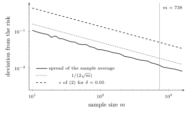
Fig. 1 shows this for the frost warning:
the sample average of the $0/1$ loss of one fixed
hypothesis, computed on samples of $\samplesize = 10$ to
$1000$ days, scatters around the risk $0.118$ with a spread
that falls like $1/\sqrt{\samplesize}$.
pythondemos/samplesize.py
For training, the same question has a second answer. The hypothesis is then chosen by looking at the sample, so the bound \(\eqref{equ_samplesize_hoeffding_dict}\) for a fixed hypothesis no longer applies to the learned one. The sample size then has to be compared with the size of the model. For a model of Vapnik–Chervonenkis dimension (VC dimension) $d$, a sample size proportional to $d / \epsilon^{2}$ makes the training error of every hypothesis in the model lie within $\epsilon$ of its risk at once (Shalev-Shwartz and Ben-David, 2014, Thm. 6.8). A sample that is small against the effective dimension of the model is the typical cause of overfitting, and the learning curve shows the validation error of the learned hypothesis as a function of the sample size (Hastie et al., 2009, Sect. 7.10).
B-dependentThe sample sizes above assume i.i.d. RVs. Data points recorded in sequence, such as consecutive days, often show autocorrelation: a frost day is more likely after a frost day, and so is a wrong prediction. Dependent data points carry less information than independent ones. For a stationary sequence with autocorrelation $\rho_{\lagidx}$ at lag $\lagidx$, the variance of the average of $\samplesize$ consecutive values is that of $\samplesize$ independent values multiplied by \begin{equation} \label{equ_samplesize_acf_dict} 1 + 2 \sum_{\lagidx=1}^{\samplesize-1} \Big( 1 - \frac{\lagidx}{\samplesize} \Big) \rho_{\lagidx} \text{,} \end{equation} see (Brockwell and Davis, 1991, Sect. 7.1). The average is therefore as accurate as that of $\samplesize$ divided by \(\eqref{equ_samplesize_acf_dict}\) independent values, the effective sample size. For the $0/1$ loss of the frost warning, the sample autocorrelation of consecutive days is $0.24$ at lag $1$ and stays positive for a week, and the factor \(\eqref{equ_samplesize_acf_dict}\) is $4.2$ for $\samplesize = 30$. The average over $30$ consecutive days therefore scatters as much as that over $7$ days drawn at random: a month of consecutive days is worth a week of random ones. A sample of consecutive data points must then be larger than \(\eqref{equ_samplesize_choice_dict}\) or \(\eqref{equ_samplesize_corr_dict}\) say, by the factor \(\eqref{equ_samplesize_acf_dict}\), or be drawn at random from the whole record, as the days of Fig. 1 are.
B-corrSample size enters a third task, hypothesis testing: are two
features of a data point correlated? For the days of
2024 at Krems, is the minimum temperature of a day correlated with
its diurnal range, the maximum minus the minimum? Over the whole
year, the Pearson correlation coefficient of the two features is
$\rho = 0.16$. A test sees a sample of $\samplesize$ days
and computes the sample correlation $r$, a function of
sample means. Under the hypothesis that the two features are uncorrelated,
$r$ scatters around $0$ with a standard deviation close to
$1/\sqrt{\samplesize}$, whatever their probability distribution. For
features that are Gaussian random variables (Gaussian RVs), Fisher's transformation
$\operatorname{artanh}(r)$ is approximately a Gaussian RV with
mean $\operatorname{artanh}(\rho)$ and standard deviation
$1/\sqrt{\samplesize - 3}$ (Fisher, 1921). The test rejects
"uncorrelated" when $|\operatorname{artanh}(r)| \sqrt{\samplesize - 3}$
exceeds the quantile $z_{1-\alpha/2}$ of the standard
Gaussian RV, which bounds the probability of a false
rejection by the significance level $\alpha$. A correlation $\rho$
is then detected with probability at least $1 - \beta$, the
power of the test, once
\begin{equation}
\label{equ_samplesize_corr_dict}
\samplesize \geq 3 + \bigg( \frac{z_{1-\alpha/2} + z_{1-\beta}}
{\operatorname{artanh}(\rho)} \bigg)^{2} \text{.}
\end{equation}
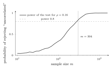
For $\rho = 0.16$, $\alpha = 0.05$ ($z_{0.975} = 1.96$) and a
power of $0.8$ ($z_{0.8} = 0.84$), the sample size
\(\eqref{equ_samplesize_corr_dict}\) is $304$ days. Fig. 2
shows the power of the test against the sample size: $0.84$ at
$\samplesize = 304$, and $0.10$ for a sample of $30$ days.
The shape is that of \(\eqref{equ_samplesize_choice_dict}\) again:
halving the correlation to be detected quadruples the sample size,
so a weak correlation needs a large sample before
"uncorrelated" can be rejected.
pythondemos/samplesize.py
See also: sample, data point, dataset, independent and identically distributed assumption, risk, empirical risk, law of large numbers, concentration inequality, Hoeffding's inequality, validation, validation error, Vapnik–Chervonenkis dimension, learning curve, overfitting, autocorrelation, hypothesis testing, Pearson correlation coefficient.
@misc{dictml_samplesize,
  author = {Jung, Alexander},
  editor = {Olioumtsevits, Konstantina and Schnoor, Ekkehard},
  title = {sample size},
  howpublished = {Dictionary of Applied Machine Learning (course edition)},
  year = {2026},
  doi = {10.5281/zenodo.21569296},
  note = {ISBN 978-952-64-3013-3, CC BY 4.0, retrieved 2026-10-14},
  url = {https://dictionaryofml.org/terms/samplesize.html}
}