B-corr writes when the script runsDictionary of Applied Machine Learning · sample size
Numerical companion to the entry sample size: it recomputes what the entry states and prints one line per check
Backs the entry's chain of claims on the frost-warning hypothesis of Krems an der Donau: a hypothesis is evaluated by its expected loss (the risk) under the i.i.d. assumption, a method sees only a sample and estimates the risk by a sample average, the gap between the two shrinks with the sample size at the rate Hoeffding's inequality states, and that inequality turns a required accuracy and confidence into a sample size. Self- contained (numpy/matplotlib only, stdlib urllib for the download), fixed seed.
Run it without installing anything:uv run https://dictionaryofml.org/terms/samplesize.py
uv downloads this script and the pinned NumPy and Matplotlib it needs, then runs it; the script fetches any input file it uses. To keep the output files, download samplesize.py into a folder and run uv run samplesize.py there. With NumPy and Matplotlib already installed, python3 samplesize.py, from any directory — it writes its output files into the current directory. Fixed seeds, so the printed numbers reproduce exactly. Download samplesize.py · Notebook · Open in Colab
One cell per block of the script: the code, and what that code printed when it last ran here
"""
samplesize.py — numerical companion to the glossary entry 'sample size'.

Purpose
-------
Backs the entry's chain of claims on the frost-warning hypothesis of Krems
an der Donau: a hypothesis is evaluated by its expected loss (the risk)
under the i.i.d. assumption, a method sees only a sample and estimates
the risk by a sample average, the gap between the two shrinks with the
sample size at the rate Hoeffding's inequality states, and that inequality
turns a required accuracy and confidence into a sample size.  Self-
contained (numpy/matplotlib only, stdlib urllib for the download), fixed
seed.

Setup
-----
Daily minimum and maximum temperature of 2024 at Krems (GeoSphere
Austria).  A data point is one day: features (minimum, maximum), label 1
if the next day's minimum is below 0 degrees (frost) and -1 otherwise.
The hypothesis under evaluation is fixed before any sampling: it predicts
frost whenever the day's minimum is below 1 degree.  The 0/1 loss of this
hypothesis on the 365 days defines the population; its average over all
days plays the role of the risk, and a sample of size m is m days drawn
uniformly with replacement, so the sampled losses are i.i.d. RVs.

Blocks
------
[B-risk]    The hypothesis, its 0/1 loss on every day, and the risk (the
            loss averaged over the whole year).
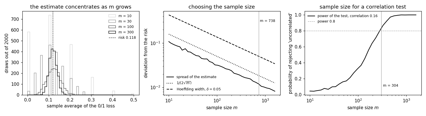
[B-sample]  Samples of size m = 10, 30, 100, 300: the sample average of
            the loss estimates the risk; over 2000 draws the largest
            deviation shrinks as m grows, and the spread of the estimate
            falls like 1/sqrt(m).
[B-bound]   Hoeffding: the fraction of draws with a deviation above
            epsilon never exceeds 2 exp(-2 m epsilon^2); the bound is
            loose but has the right shape.
[B-choose]  Sample size from the bound: a deviation of at most 0.05 with
            probability at least 0.95 needs m >= log(2/0.05) / (2 0.05^2)
            = 738 days, and the empirical rate at m = 738 confirms it.
[B-dependent] Consecutive days are not i.i.d.: the 0/1 loss of the
            hypothesis has sample autocorrelation 0.24 at lag 1 (a wrong
            prediction follows a wrong prediction).  The variance of the
            average over m consecutive days is that over m random days
            times 1 + 2 sum_k (1 - k/m) rho_k; for m = 30 the factor is
            4.2 and the measured ratio 4.4, so 30 consecutive days are
            worth 7 random ones: the effective sample size.
[B-corr]    Sample size for a statistical test: are two features of a day,
            its minimum temperature and its diurnal range (maximum minus
            minimum), correlated?  Over the year the Pearson correlation
            coefficient is 0.16.  With the features uncorrelated, the
            sample correlation r scatters around 0 with standard deviation
            1/sqrt(m) and the test "reject 'uncorrelated' when
            |artanh(r)| sqrt(m - 3) > 1.96" rejects with frequency 0.05;
            detecting 0.16 with probability 0.8 needs
            m >= 3 + ((1.96 + 0.84) / artanh(0.16))^2 = 304 days (Fisher's
            formula for Gaussian features): the empirical power is 0.84
            there and 0.10 at m = 30.

Outputs
-------
samplesize_losses.csv   : day, minimum, maximum, label, loss of the hypothesis
samplesize_curve.csv    : m, sample standard deviation of the estimate,
                          1/(2 sqrt m), Hoeffding width for delta = 0.05
samplesize_bound.csv    : m, epsilon, empirical tail probability, Hoeffding
                          bound
samplesize_corr.csv     : m, standard deviation of artanh(r), 1/sqrt(m - 3),
                          power of the correlation test at level 0.05
samplesize_acf.csv      : lag, sample autocorrelation of the loss sequence
samplesize.png          : matplotlib preview (checking only)
"""

import json
import math
import urllib.request

import numpy as np
import matplotlib

matplotlib.use("Agg")
import matplotlib.pyplot as plt

from pathlib import Path

OUT_DIR = Path(__file__).parent

report = []


def check(name, ok):
    report.append((name, bool(ok)))
    print(f"  [{'ok' if ok else 'FAIL'}] {name}")
The hypothesis, its 0/1 loss on every day, and the risk (the loss averaged over the whole year).
URL = ("https://dataset.api.hub.geosphere.at/v1/station/historical/"
       "klima-v2-1d?parameters=tlmin,tlmax&station_ids=3805"
       "&start=2024-01-01&end=2024-12-31")
with urllib.request.urlopen(URL, timeout=120) as resp:
    payload = json.load(resp)
par = payload["features"][0]["properties"]["parameters"]
tmin = np.array(par["tlmin"]["data"], dtype=float)
tmax = np.array(par["tlmax"]["data"], dtype=float)
days = [s[:10] for s in payload["timestamps"]]
x = np.c_[tmin[:-1], tmax[:-1]]                 # a day's two features
y = np.where(tmin[1:] < 0.0, 1, -1)             # frost on the following day
N = len(y)
THRESH = 1.0
pred = np.where(x[:, 0] < THRESH, 1, -1)        # the fixed hypothesis
loss = (pred != y).astype(float)                # 0/1 loss per day
risk = float(loss.mean())
check(f"[B-risk]    {N} days of 2024, {int((y == 1).sum())} followed by frost; the hypothesis "
      f"'frost if today's minimum is below {THRESH:g} degrees' has risk {risk:.3f} "
      f"(its 0/1 loss averaged over the year)", 0.0 < risk < 0.5)
with open(OUT_DIR / "samplesize_losses.csv", "w") as fh:
    fh.write("day,tmin,tmax,label,loss\n")
    for d, xi, yi, li in zip(days[:-1], x, y, loss):
        fh.write(f"{d},{xi[0]:g},{xi[1]:g},{yi},{int(li)}\n")
  [ok] [B-risk]    365 days of 2024, 68 followed by frost; the hypothesis 'frost if today's minimum is below 1 degrees' has risk 0.118 (its 0/1 loss averaged over the year)
    sample size m, largest |estimate - risk| over 2000 draws, spread of the estimate:
      m =    10: largest deviation 0.382, standard deviation 0.1043
      m =    30: largest deviation 0.249, standard deviation 0.0583
      m =   100: largest deviation 0.102, standard deviation 0.0319
      m =   300: largest deviation 0.072, standard deviation 0.0185
      m =  1000: largest deviation 0.035, standard deviation 0.0103
Samples of size m = 10, 30, 100, 300: the sample average of the loss estimates the risk; over 2000 draws the largest deviation shrinks as m grows, and the spread of the estimate falls like 1/sqrt(m).
rng = np.random.default_rng(2024)
SIZES = [10, 30, 100, 300, 1000]
DRAWS = 2000
est = {m: loss[rng.integers(0, N, (DRAWS, m))].mean(axis=1) for m in SIZES}
dev = {m: np.abs(est[m] - risk) for m in SIZES}
sd = {m: float(est[m].std()) for m in SIZES}
print("    sample size m, largest |estimate - risk| over 2000 draws, spread of the estimate:")
for m in SIZES:
    print(f"      m = {m:5d}: largest deviation {dev[m].max():.3f}, standard deviation {sd[m]:.4f}")
check("[B-sample]  the sample average of the loss estimates the risk, and its largest "
      "deviation over 2000 draws shrinks with m",
      all(dev[a].max() > dev[b].max() for a, b in zip(SIZES, SIZES[1:])))
ratio = [sd[m] * math.sqrt(m) for m in SIZES]
check(f"[B-sample]  the spread of the estimate falls like 1/sqrt(m): sd * sqrt(m) stays near "
      f"{np.mean(ratio):.2f} ({min(ratio):.2f} to {max(ratio):.2f})",
      max(ratio) - min(ratio) < 0.1)
  [ok] [B-sample]  the sample average of the loss estimates the risk, and its largest deviation over 2000 draws shrinks with m
  [ok] [B-sample]  the spread of the estimate falls like 1/sqrt(m): sd * sqrt(m) stays near 0.32 (0.32 to 0.33)
Hoeffding: the fraction of draws with a deviation above epsilon never exceeds 2 exp(-2 m epsilon^2); the bound is loose but has the right shape.
EPS = [0.05, 0.1, 0.15]
rows = []
for m in SIZES:
    for eps in EPS:
        emp = float(np.mean(dev[m] > eps))
        bnd = min(1.0, 2.0 * math.exp(-2.0 * m * eps ** 2))
        rows.append((m, eps, emp, bnd))
check("[B-bound]   Hoeffding: the fraction of draws with a deviation above epsilon never exceeds "
      "2 exp(-2 m epsilon^2), for every m and epsilon", all(emp <= bnd + 1e-12 for _, _, emp, bnd in rows))
with open(OUT_DIR / "samplesize_bound.csv", "w") as fh:
    fh.write("m,epsilon,empirical,hoeffding\n")
    for m, eps, emp, bnd in rows:
        fh.write(f"{m},{eps},{emp:.4f},{bnd:.4f}\n")
[ok] [B-bound] Hoeffding: the fraction of draws with a deviation above epsilon never exceeds 2 exp(-2 m epsilon^2), for every m and epsilon
Sample size from the bound: a deviation of at most 0.05 with probability at least 0.95 needs m >= log(2/0.05) / (2 0.05^2) = 738 days, and the empirical rate at m = 738 confirms it.
EPS0, DELTA = 0.05, 0.05
m_needed = math.ceil(math.log(2.0 / DELTA) / (2.0 * EPS0 ** 2))
est_needed = loss[rng.integers(0, N, (DRAWS, m_needed))].mean(axis=1)
rate = float(np.mean(np.abs(est_needed - risk) <= EPS0))
check(f"[B-choose]  a deviation of at most {EPS0} with probability at least {1 - DELTA} needs "
      f"m >= log(2/{DELTA}) / (2 * {EPS0}^2) = {m_needed} days; at that size "
      f"{rate:.3f} of 2000 draws are within {EPS0}", rate >= 1 - DELTA)
grid = np.unique(np.round(np.logspace(1, 3.2, 40)).astype(int))
with open(OUT_DIR / "samplesize_curve.csv", "w") as fh:
    fh.write("m,sd,halfsqrt,hoeffding\n")
    for m in grid:
        s = float(loss[rng.integers(0, N, (400, m))].mean(axis=1).std())
        fh.write(f"{m},{s:.4f},{1 / (2 * math.sqrt(m)):.4f},{math.sqrt(math.log(2 / DELTA) / (2 * m)):.4f}\n")
  [ok] [B-choose]  a deviation of at most 0.05 with probability at least 0.95 needs m >= log(2/0.05) / (2 * 0.05^2) = 738 days; at that size 1.000 of 2000 draws are within 0.05
    sample autocorrelation of the loss at lags 1 to 7: 0.24, 0.11, 0.24, 0.11, 0.19, 0.16, 0.08
      m = 30: variance ratio consecutive / random 4.31, factor 1 + 2 sum (1 - k/m) rho_k = 4.19, effective sample size 7
      m = 60: variance ratio consecutive / random 5.80, factor 1 + 2 sum (1 - k/m) rho_k = 6.11, effective sample size 10
Consecutive days are not i.i.d.: the 0/1 loss of the hypothesis has sample autocorrelation 0.24 at lag 1 (a wrong prediction follows a wrong prediction). The variance of the average over m consecutive days is that over m random days times 1 + 2 sum_k (1 - k/m) rho_k; for m = 30 the factor is 4.2 and the measured ratio 4.4, so 30 consecutive days are worth 7 random ones: the effective sample size.
def acf(v, k):
    v = v - v.mean()
    return float((v[:-k] * v[k:]).sum() / (v * v).sum())


rhos = [acf(loss, k) for k in range(1, 61)]
print("    sample autocorrelation of the loss at lags 1 to 7: "
      + ", ".join(f"{r:.2f}" for r in rhos[:7]))
dep = {}
for m in (30, 60):
    windows = np.array([loss[i:i + m].mean() for i in range(N - m + 1)])   # consecutive days
    random_ = loss[rng.integers(0, N, (4000, m))].mean(1)                   # days drawn at random
    factor = 1 + 2 * sum((1 - k / m) * rhos[k - 1] for k in range(1, m))
    dep[m] = (windows.var() / random_.var(), factor, m / factor)
    print(f"      m = {m}: variance ratio consecutive / random {dep[m][0]:.2f}, "
          f"factor 1 + 2 sum (1 - k/m) rho_k = {factor:.2f}, effective sample size {m / factor:.0f}")
check(f"[B-dependent] the loss of consecutive days is autocorrelated, rho_1 = {rhos[0]:.2f}, "
      f"and the average over m consecutive days has the variance of m random days times "
      f"1 + 2 sum (1 - k/m) rho_k, to within 25% at m = 30 and 60",
      rhos[0] > 0.15 and all(abs(r / f - 1) < 0.25 for r, f, _ in dep.values()))
check(f"[B-dependent] 30 consecutive days are worth {dep[30][2]:.0f} random ones (effective sample size)",
      5 <= dep[30][2] <= 9)
with open(OUT_DIR / "samplesize_acf.csv", "w") as fh:
    fh.write("lag,rho\n")
    for k, r in enumerate(rhos[:30], 1):
        fh.write(f"{k},{r:.4f}\n")
  [ok] [B-dependent] the loss of consecutive days is autocorrelated, rho_1 = 0.24, and the average over m consecutive days has the variance of m random days times 1 + 2 sum (1 - k/m) rho_k, to within 25% at m = 30 and 60
  [ok] [B-dependent] 30 consecutive days are worth 7 random ones (effective sample size)
    minimum temperature and diurnal range: correlation 0.160 over the 365 days
Sample size for a statistical test: are two features of a day, its minimum temperature and its diurnal range (maximum minus minimum), correlated? Over the year the Pearson correlation coefficient is 0.16. With the features uncorrelated, the sample correlation r scatters around 0 with standard deviation 1/sqrt(m) and the test "reject 'uncorrelated' when |artanh(r)| sqrt(m - 3) > 1.96" rejects with frequency 0.05; detecting 0.16 with probability 0.8 needs m >= 3 + ((1.96 + 0.84) / artanh(0.16))^2 = 304 days (Fisher's formula for Gaussian features): the empirical power is 0.84 there and 0.10 at m = 30.
def gauss_quantile(p):
    """The standard Gaussian quantile, by bisection on the cdf."""
    lo, hi = -10.0, 10.0
    for _ in range(100):
        mid = 0.5 * (lo + hi)
        if 0.5 * (1.0 + math.erf(mid / math.sqrt(2.0))) < p:
            lo = mid
        else:
            hi = mid
    return 0.5 * (lo + hi)


ALPHA, POWER = 0.05, 0.8
z_alpha, z_power = gauss_quantile(1 - ALPHA / 2), gauss_quantile(POWER)
f1, f2 = x[:, 0], x[:, 1] - x[:, 0]                # two features of the 365 labeled days
rho = float(np.corrcoef(f1, f2)[0, 1])
m_corr = math.ceil(3 + ((z_alpha + z_power) / math.atanh(rho)) ** 2)


def sample_corr(a, b, m, draws):
    idx = rng.integers(0, len(a), (draws, m))
    aa, bb = a[idx], b[idx]
    aa = aa - aa.mean(1, keepdims=True); bb = bb - bb.mean(1, keepdims=True)
    return (aa * bb).sum(1) / np.sqrt((aa ** 2).sum(1) * (bb ** 2).sum(1))


def power_at(m, draws=2000):
    r = sample_corr(f1, f2, m, draws)
    return float(np.mean(np.abs(np.arctanh(r)) * math.sqrt(m - 3) > z_alpha))


print(f"    minimum temperature and diurnal range: correlation {rho:.3f} over the {len(f1)} days")


def null_corr(m, draws):
    """Sample correlation of the two features drawn independently: uncorrelated by construction."""
    a = f1[rng.integers(0, len(f1), (draws, m))]; b = f2[rng.integers(0, len(f2), (draws, m))]
    a = a - a.mean(1, keepdims=True); b = b - b.mean(1, keepdims=True)
    return (a * b).sum(1) / np.sqrt((a ** 2).sum(1) * (b ** 2).sum(1))


nsd = {m: float(null_corr(m, 2000).std() * math.sqrt(m)) for m in (30, 100, 300, 1000)}
check("[B-corr]    with the two features uncorrelated, the sample correlation r scatters around 0 "
      "with standard deviation close to 1/sqrt(m): sd * sqrt(m) = "
      + ", ".join(f"{v:.2f} (m = {m})" for m, v in nsd.items()), all(0.88 < v < 1.12 for v in nsd.values()))
size = float(np.mean(np.abs(np.arctanh(null_corr(100, 4000))) * math.sqrt(97) > z_alpha))
check(f"[B-corr]    on uncorrelated features the test rejects at level {ALPHA} with frequency "
      f"{size:.3f}", size < 0.075)
zsd = {m: float(np.arctanh(sample_corr(f1, f2, m, 2000)).std() * math.sqrt(m - 3)) for m in (30, 300, 1000)}
print("    at rho = 0.16, sd of artanh(r) times sqrt(m - 3): "
      + ", ".join(f"{v:.2f} (m = {m})" for m, v in zsd.items()) + " (1 for Gaussian features)")
p_small, p_need = power_at(30), power_at(m_corr)
check(f"[B-corr]    detecting rho = {rho:.2f} at level {ALPHA} with power {POWER} needs "
      f"m >= 3 + (({z_alpha:.2f} + {z_power:.2f}) / artanh({rho:.2f}))^2 = {m_corr} days; empirical power "
      f"{p_need:.2f} at m = {m_corr}, only {p_small:.2f} at m = 30",
      abs(p_need - POWER) < 0.08 and p_small < 0.3)
with open(OUT_DIR / "samplesize_corr.csv", "w") as fh:
    fh.write("m,zsd,invsqrt,power\n")
    for m in np.unique(np.round(np.logspace(1, 3.2, 30)).astype(int)):
        r = sample_corr(f1, f2, int(m), 1000)
        fh.write(f"{m},{np.arctanh(r).std():.4f},{1 / math.sqrt(m - 3):.4f},"
                 f"{np.mean(np.abs(np.arctanh(r)) * math.sqrt(m - 3) > z_alpha):.3f}\n")

# -------------------------------------------------------------- preview
fig, (ax1, ax2, ax3) = plt.subplots(1, 3, figsize=(13.5, 3.7))
for m, c in zip(SIZES[:4], ("0.85", "0.6", "0.35", "0.0")):
    ax1.hist(est[m], bins=np.linspace(0, 0.5, 51), histtype="step", color=c, label=f"m = {m}")
ax1.axvline(risk, color="k", ls="--", lw=0.8, label=f"risk {risk:.3f}")
ax1.set_xlabel("sample average of the 0/1 loss"); ax1.set_ylabel("draws out of 2000")
ax1.set_title("the estimate concentrates as m grows"); ax1.legend(frameon=False, fontsize=8)
cv = np.genfromtxt(OUT_DIR / "samplesize_curve.csv", delimiter=",", names=True)
ax2.loglog(cv["m"], cv["sd"], "k-", label="spread of the estimate")
ax2.loglog(cv["m"], cv["halfsqrt"], "k:", label=r"$1/(2\sqrt{m})$")
ax2.loglog(cv["m"], cv["hoeffding"], "k--", label=r"Hoeffding width, $\delta = 0.05$")
ax2.axvline(m_needed, color="0.6", lw=0.8); ax2.text(m_needed * 1.05, 0.3, f"m = {m_needed}", fontsize=8)
ax2.set_xlabel("sample size $m$"); ax2.set_ylabel("deviation from the risk")
ax2.set_title("choosing the sample size"); ax2.legend(frameon=False, fontsize=8)
cc = np.genfromtxt(OUT_DIR / "samplesize_corr.csv", delimiter=",", names=True)
ax3.semilogx(cc["m"], cc["power"], "k-", label=f"power of the test, correlation {rho:.2f}")
ax3.axhline(POWER, color="0.6", lw=0.8, ls="--", label=f"power {POWER}")
ax3.axvline(m_corr, color="0.6", lw=0.8); ax3.text(m_corr * 1.08, 0.1, f"m = {m_corr}", fontsize=8)
ax3.set_xlabel("sample size $m$"); ax3.set_ylabel("probability of rejecting 'uncorrelated'")
ax3.set_title("sample size for a correlation test"); ax3.legend(frameon=False, fontsize=8)
fig.tight_layout()
fig.savefig(OUT_DIR / "samplesize.png", dpi=110)

n_ok = sum(ok for _, ok in report)
print(f"\n{n_ok}/{len(report)} checks pass")
print(f"wrote {OUT_DIR / 'samplesize_losses.csv'}, {OUT_DIR / 'samplesize_curve.csv'}, "
      f"{OUT_DIR / 'samplesize_bound.csv'}, {OUT_DIR / 'samplesize_corr.csv'}, "
      f"{OUT_DIR / 'samplesize_acf.csv'}, {OUT_DIR / 'samplesize.png'}")
if n_ok != len(report):
    raise SystemExit(1)
  [ok] [B-corr]    with the two features uncorrelated, the sample correlation r scatters around 0 with standard deviation close to 1/sqrt(m): sd * sqrt(m) = 0.98 (m = 30), 1.02 (m = 100), 1.02 (m = 300), 1.00 (m = 1000)
  [ok] [B-corr]    on uncorrelated features the test rejects at level 0.05 with frequency 0.049
    at rho = 0.16, sd of artanh(r) times sqrt(m - 3): 0.85 (m = 30), 0.83 (m = 300), 0.84 (m = 1000) (1 for Gaussian features)
  [ok] [B-corr]    detecting rho = 0.16 at level 0.05 with power 0.8 needs m >= 3 + ((1.96 + 0.84) / artanh(0.16))^2 = 304 days; empirical power 0.84 at m = 304, only 0.10 at m = 30

10/10 checks pass
wrote /Users/junga1/dictionaryappliedml/pythondemos/samplesize_losses.csv, /Users/junga1/dictionaryappliedml/pythondemos/samplesize_curve.csv, /Users/junga1/dictionaryappliedml/pythondemos/samplesize_bound.csv, /Users/junga1/dictionaryappliedml/pythondemos/samplesize_corr.csv, /Users/junga1/dictionaryappliedml/pythondemos/samplesize_acf.csv, /Users/junga1/dictionaryappliedml/pythondemos/samplesize.png
B-corr writes when the script runs